
Bioinformatics is the science of transforming and processing biological data to gain new insights, particularly omics data: genomics, proteomics, metabolomics, etc.. Bioinformatics is mostly a mix of biology, computer science, and statistics / data science.
A k-mer is a substring of length k within some larger biological sequence (e.g. DNA or amino acid chain). For example, in the DNA sequence GAAATC, the following k-mer's exist:
| k | k-mers |
|---|---|
| 1 | G A A A T C |
| 2 | GA AA AA AT TC |
| 3 | GAA AAA AAT ATC |
| 4 | GAAA AAAT AATC |
| 5 | GAAAT AAATC |
| 6 | GAAATC |
Common scenarios involving k-mers:
WHAT: Given a DNA k-mer, calculate its reverse complement.
WHY: Depending on the type of biological sequence, a k-mer may have one or more alternatives. For DNA sequences specifically, a k-mer of interest may have an alternate form. Since the DNA molecule comes as 2 strands, where ...
, ... the reverse complement of that k-mer may be just as valid as the original k-mer. For example, if an enzyme is known to bind to a specific DNA k-mer, it's possible that it might also bind to the reverse complement of that k-mer.
ALGORITHM:
ch1_code/src/ReverseComplementADnaKmer.py (lines 5 to 22):
def reverse_complement(strand: str):
    ret = ''
    for i in range(0, len(strand)):
        base = strand[i]
        if base == 'A' or base == 'a':
            base = 'T'
        elif base == 'T' or base == 't':
            base = 'A'
        elif base == 'C' or base == 'c':
            base = 'G'
        elif base == 'G' or base == 'g':
            base = 'C'
        else:
            raise Exception('Unexpected base: ' + base)

        ret += base
    return ret[::-1]
Original: TAATCCG
Reverse Complement: CGGATTA
WHAT: Given 2 k-mers, the hamming distance is the number of positional mismatches between them.
WHY: Imagine an enzyme that looks for a specific DNA k-mer pattern to bind to. Since DNA is known to mutate, it may be that enzyme can also bind to other k-mer patterns that are slight variations of the original. For example, that enzyme may be able to bind to both AAACTG and AAAGTG.
ALGORITHM:
ch1_code/src/HammingDistanceBetweenKmers.py (lines 5 to 13):
def hamming_distance(kmer1: str, kmer2: str) -> int:
    mismatch = 0

    for ch1, ch2 in zip(kmer1, kmer2):
        if ch1 != ch2:
            mismatch += 1

    return mismatch
Kmer1: ACTTTGTT
Kmer2: AGTTTCTT
Hamming Distance: 2
↩PREREQUISITES↩
WHAT: Given a source k-mer and a minimum hamming distance, find all k-mers such within the hamming distance of the source k-mer. In other words, find all k-mers such that hamming_distance(source_kmer, kmer) <= min_distance.
WHY: Imagine an enzyme that looks for a specific DNA k-mer pattern to bind to. Since DNA is known to mutate, it may be that enzyme can also bind to other k-mer patterns that are slight variations of the original. This algorithm finds all such variations.
ALGORITHM:
ch1_code/src/FindAllDnaKmersWithinHammingDistance.py (lines 5 to 20):
def find_all_dna_kmers_within_hamming_distance(kmer: str, hamming_dist: int) -> set[str]:
    def recurse(kmer: str, hamming_dist: int, output: set[str]) -> None:
        if hamming_dist == 0:
            output.add(kmer)
            return

        for i in range(0, len(kmer)):
            for ch in 'ACTG':
                neighbouring_kmer = kmer[:i] + ch + kmer[i + 1:]
                recurse(neighbouring_kmer, hamming_dist - 1, output)

    output = set()
    recurse(kmer, hamming_dist, output)

    return output
Kmers within hamming distance 1 of AAAA: {'ATAA', 'AACA', 'AAAC', 'GAAA', 'ACAA', 'AAAT', 'CAAA', 'AAAG', 'AGAA', 'AAGA', 'AATA', 'TAAA', 'AAAA'}
↩PREREQUISITES↩
WHAT: Given a k-mer, find where that k-mer occurs in some larger sequence. The search may potentially include the k-mer's variants (e.g. reverse complement).
WHY: Imagine that you know of a specific k-mer pattern that serves some function in an organism. If you see that same k-mer pattern appearing in some other related organism, it could be a sign that k-mer pattern serves a similar function. For example, the same k-mer pattern could be used by 2 related types of bacteria as a DnaA box.
The enzyme that operates on that k-mer may also operate on its reverse complement as well as slight variations on that k-mer. For example, if an enzyme binds to AAAAAAAAA, it may also bind to its...
ALGORITHM:
ch1_code/src/FindLocations.py (lines 11 to 32):
class Options(NamedTuple):
    hamming_distance: int = 0
    reverse_complement: bool = False


def find_kmer_locations(sequence: str, kmer: str, options: Options = Options()) -> List[int]:
    # Construct test kmers
    test_kmers = set()
    test_kmers.add(kmer)
    [test_kmers.add(alt_kmer) for alt_kmer in find_all_dna_kmers_within_hamming_distance(kmer, options.hamming_distance)]
    if options.reverse_complement:
        rc_kmer = reverse_complement(kmer)
        [test_kmers.add(alt_rc_kmer) for alt_rc_kmer in find_all_dna_kmers_within_hamming_distance(rc_kmer, options.hamming_distance)]

    # Slide over the sequence's kmers and check for matches against test kmers
    k = len(kmer)
    idxes = []
    for seq_kmer, i in slide_window(sequence, k):
        if seq_kmer in test_kmers:
            idxes.append(i)
    return idxes
Found AAAA in AAAAGAACCTAATCTTAAAGGAGATGATGATTCTAA at index [0, 1, 2, 3, 12, 15, 16, 30]
↩PREREQUISITES↩
WHAT: Given a k-mer, find where that k-mer clusters in some larger sequence. The search may potentially include the k-mer's variants (e.g. reverse complement).
WHY: An enzyme may need to bind to a specific region of DNA to begin doing its job. That is, it looks for a specific k-mer pattern to bind to, where that k-mer represents the beginning of some larger DNA region that it operates on. Since DNA is known to mutate, oftentimes you'll find multiple copies of the same k-mer pattern clustered together -- if one copy mutated to become unusable, the other copies are still around.
For example, the DnaA box is a special k-mer pattern used by enzymes during DNA replication. Since DNA is known to mutate, the DnaA box can be found repeating multiple times in the region of DNA known as the replication origin. Finding the DnaA box clustered in a small region is a good indicator that you've found the replication origin.
ALGORITHM:
ch1_code/src/FindClumps.py (lines 10 to 26):
def find_kmer_clusters(sequence: str, kmer: str, min_occurrence_in_cluster: int, cluster_window_size: int, options: Options = Options()) -> List[int]:
    cluster_locs = []

    locs = find_kmer_locations(sequence, kmer, options)
    start_i = 0
    occurrence_count = 1
    for end_i in range(1, len(locs)):
        if locs[end_i] - locs[start_i] < cluster_window_size:  # within a cluster window?
            occurrence_count += 1
        else:
            if occurrence_count >= min_occurrence_in_cluster:  # did the last cluster meet the min ocurr requirement?
                cluster_locs.append(locs[start_i])
            start_i = end_i
            occurrence_count = 1

    return cluster_locs
Found clusters of GGG (at least 3 occurrences in window of 13) in GGGACTGAACAAACAAATTTGGGAGGGCACGGGTTAAAGGAGATGATGATTCAAAGGGT at index [19, 37]
WHAT: Given a sequence, find clusters of unique k-mers within that sequence. In other words, for each unique k-mer that exists in the sequence, see if it clusters in the sequence. The search may potentially include variants of k-mer variants (e.g. reverse complements of the k-mers).
WHY: An enzyme may need to bind to a specific region of DNA to begin doing its job. That is, it looks for a specific k-mer pattern to bind to, where that k-mer represents the beginning of some larger DNA region that it operates on. Since DNA is known to mutate, oftentimes you'll find multiple copies of the same k-mer pattern clustered together -- if one copy mutated to become unusable, the other copies are still around.
For example, the DnaA box is a special k-mer pattern used by enzymes during DNA replication. Since DNA is known to mutate, the DnaA box can be found repeating multiple times in the region of DNA known as the replication origin. Given that you don't know the k-mer pattern for the DnaA box but you do know the replication origin, you can scan through the replication origin for repeating k-mer patterns. If a pattern is found to heavily repeat, it's a good candidate that it's the k-mer pattern for the DnaA box.
ALGORITHM:
ch1_code/src/FindRepeating.py (lines 12 to 41):
from Utils import slide_window


def count_kmers(data: str, k: int, options: Options = Options()) -> Counter[str]:
    counter = Counter()
    for kmer, i in slide_window(data, k):
        neighbourhood = find_all_dna_kmers_within_hamming_distance(kmer, options.hamming_distance)
        for neighbouring_kmer in neighbourhood:
            counter[neighbouring_kmer] += 1

        if options.reverse_complement:
            kmer_rc = reverse_complement(kmer)
            neighbourhood = find_all_dna_kmers_within_hamming_distance(kmer_rc, options.hamming_distance)
            for neighbouring_kmer in neighbourhood:
                counter[neighbouring_kmer] += 1

    return counter


def top_repeating_kmers(data: str, k: int, options: Options = Options()) -> Set[str]:
    counts = count_kmers(data, k, options)

    _, top_count = counts.most_common(1)[0]

    top_kmers = set()
    for kmer, count in counts.items():
        if count == top_count:
            top_kmers.add((kmer, count))
    return top_kmers
Top 5-mer frequencies for GGGACTGAACAAACAAATTTGGGAGGGCACGGGTTAAAGGAGATGATGATTCAAAGGGT:
↩PREREQUISITES↩
WHAT: Given a sequence, find regions within that sequence that contain clusters of unique k-mers. In other words, ...
The search may potentially include variants of k-mer variants (e.g. reverse complements of the k-mers).
WHY: An enzyme may need to bind to a specific region of DNA to begin doing its job. That is, it looks for a specific k-mer pattern to bind to, where that k-mer represents the beginning of some larger DNA region that it operates on. Since DNA is known to mutate, oftentimes you'll find multiple copies of the same k-mer pattern clustered together -- if one copy mutated to become unusable, the other copies are still around.
For example, the DnaA box is a special k-mer pattern used by enzymes during DNA replication. Since DNA is known to mutate, the DnaA box can be found repeating multiple times in the region of DNA known as the replication origin. Given that you don't know the k-mer pattern for the DnaA box but you do know the replication origin, you can scan through the replication origin for repeating k-mer patterns. If a pattern is found to heavily repeat, it's a good candidate that it's the k-mer pattern for the DnaA box.
ALGORITHM:
ch1_code/src/FindRepeatingInWindow.py (lines 20 to 67):
def scan_for_repeating_kmers_in_clusters(sequence: str, k: int, min_occurrence_in_cluster: int, cluster_window_size: int, options: Options = Options()) -> Set[KmerCluster]:
    def neighborhood(kmer: str) -> Set[str]:
        neighbourhood = find_all_dna_kmers_within_hamming_distance(kmer, options.hamming_distance)
        if options.reverse_complement:
            kmer_rc = reverse_complement(kmer)
            neighbourhood = find_all_dna_kmers_within_hamming_distance(kmer_rc, options.hamming_distance)
        return neighbourhood

    kmer_counter = {}

    def add_kmer(kmer: str, loc: int) -> None:
        if kmer not in kmer_counter:
            kmer_counter[kmer] = set()
        kmer_counter[kmer].add(window_idx + kmer_idx)

    def remove_kmer(kmer: str, loc: int) -> None:
        kmer_counter[kmer].remove(window_idx - 1)
        if len(kmer_counter[kmer]) == 0:
            del kmer_counter[kmer]

    clustered_kmers = set()

    old_first_kmer = None
    for window, window_idx in slide_window(sequence, cluster_window_size):
        first_kmer = window[0:k]
        last_kmer = window[-k:]

        # If first iteration, add all kmers
        if window_idx == 0:
            for kmer, kmer_idx in slide_window(window, k):
                for alt_kmer in neighborhood(kmer):
                    add_kmer(alt_kmer, window_idx + kmer_idx)
        else:
            # Add kmer that was walked in to
            for new_last_kmer in neighborhood(last_kmer):
                add_kmer(new_last_kmer, window_idx + cluster_window_size - k)
            # Remove kmer that was walked out of
            if old_first_kmer is not None:
                for alt_kmer in neighborhood(old_first_kmer):
                    remove_kmer(alt_kmer, window_idx - 1)

        old_first_kmer = first_kmer

        # Find clusters within window -- tuple is k-mer, start_idx, occurrence_count
        [clustered_kmers.add(KmerCluster(k, min(v), len(v))) for k, v in kmer_counter.items() if len(v) >= min_occurrence_in_cluster]

    return clustered_kmers
Found clusters of k=9 (at least 6 occurrences in window of 20) in TTTTTTTTTTTTTCCCTTTTTTTTTCCCTTTTTTTTTTTTT at...
↩PREREQUISITES↩
WHAT: Given ...
... find the probability of that k-mer appearing at least c times within an arbitrary sequence of length n. For example, the probability that the 2-mer AA appears at least 2 times in a sequence of length 4:
The probability is 7/256.
This isn't trivial to accurately compute because the occurrences of a k-mer within a sequence may overlap. For example, the number of times AA appears in AAAA is 3 while in CAAA it's 2.
WHY: When a k-mer is found within a sequence, knowing the probability of that k-mer being found within an arbitrary sequence of the same length hints at the significance of the find. For example, if some 10-mer has a 0.2 chance of appearing in an arbitrary sequence of length 50, that's too high of a chance to consider it a significant find -- 0.2 means 1 in 5 chance that the 10-mer just randomly happens to appear.
ALGORITHM:
This algorithm tries every possible combination of sequence to find the probability. It falls over once the length of the sequence extends into the double digits. It's intended to help conceptualize what's going on.
ch1_code/src/BruteforceProbabilityOfKmerInArbitrarySequence.py (lines 9 to 39):
# Of the X sequence combinations tried, Y had the k-mer. The probability is Y/X.
def bruteforce_probability(searchspace_len: int, searchspace_symbol_count: int, search_for: List[int], min_occurrence: int) -> (int, int):
    found = 0
    found_max = searchspace_symbol_count ** searchspace_len

    str_to_search = [0] * searchspace_len

    def count_instances():
        ret = 0
        for i in range(0, searchspace_len - len(search_for) + 1):
            if str_to_search[i:i + len(search_for)] == search_for:
                ret += 1
        return ret

    def walk(idx: int):
        nonlocal found

        if idx == searchspace_len:
            count = count_instances()
            if count >= min_occurrence:
                found += 1
        else:
            for i in range(0, searchspace_symbol_count):
                walk(idx + 1)
                str_to_search[idx] += 1
            str_to_search[idx] = 0

    walk(0)

    return found, found_max
Brute-forcing probability of ACTG in arbitrary sequence of length 8
Probability: 0.0195159912109375 (1279/65536)
ALGORITHM:
⚠️NOTE️️️⚠️
The explanation in the comments below are a bastardization of "1.13 Detour: Probabilities of Patterns in a String" in the Pevzner book...
This algorithm tries estimating the probability by ignoring the fact that the occurrences of a k-mer in a sequence may overlap. For example, searching for the 2-mer AA in the sequence AAAT yields 2 instances of AA:
If you go ahead and ignore overlaps, you can think of the k-mers occurring in a string as insertions. For example, imagine a sequence of length 7 and the 2-mer AA. If you were to inject 2 instances of AA into the sequence to get it to reach length 7, how would that look?
2 instances of a 2-mer is 4 characters has a length of 5. To get the sequence to end up with a length of 7 after the insertions, the sequence needs to start with a length of 3:
SSS
Given that you're changing reality to say that the instances WON'T overlap in the sequence, you can treat each instance of the 2-mer AA as a single entity being inserted. The number of ways that these 2 instances can be inserted into the sequence is 10:
I = insertion of AA, S = arbitrary sequence character

IISSS  ISISS  ISSIS  ISSSI
SIISS  SISIS  SISSI
SSIIS  SSISI
SSSII
Another way to think of the above insertions is that they aren't insertions. Rather, you have 5 items in total and you're selecting 2 of them. How many ways can you select 2 of those 5 items? 10.
The number of ways to insert can be counted via the "binomial coefficient": bc(m, k) = m!/(k!(m-k)!), where m is the total number of items (5 in the example above) and k is the number of selections (2 in the example above). For the example above:
bc(5, 2) = 5!/(2!(5-2)!) = 10
Since the SSS can be any arbitrary nucleotide sequence of 3, count the number of different representations that are possible for SSS: 4^3 = 4*4*4 = 64 (4^3, 4 because a nucleotide can be one of ACTG, 3 because the length is 3). In each of these representations, the 2-mer AA can be inserted in 10 different ways:
64*10 = 640
Since the total length of the sequence is 7, count the number of different representations that are possible:
4^7 = 4*4*4*4*4*4*4 = 16384
The estimated probability is 640/16384. For...
⚠️NOTE️️️⚠️
Maybe try training a deep learning model to see if it can provide better estimates?
ch1_code/src/EstimateProbabilityOfKmerInArbitrarySequence.py (lines 57 to 70):
def estimate_probability(searchspace_len: int, searchspace_symbol_count: int, search_for: List[int], min_occurrence: int) -> float:
    def factorial(num):
        if num == 1:
            return num
        else:
            return num * factorial(num - 1)

    def bc(m, k):
        return factorial(m) / (factorial(k) * factorial(m - k))

    k = len(search_for)
    n = (searchspace_len - min_occurrence * k)
    return bc(n + min_occurrence, min_occurrence) * (searchspace_symbol_count ** n) / searchspace_symbol_count ** searchspace_len
Estimating probability of ACTG in arbitrary sequence of length 8
Probability: 0.01953125
WHAT: Given a sequence, create a counter and walk over the sequence. Whenever a ...
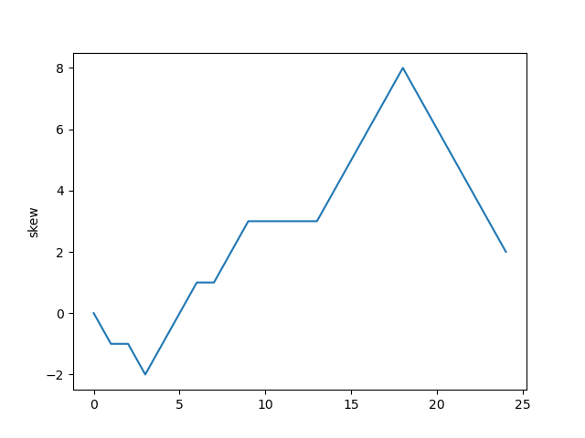
WHY: Given the DNA sequence of an organism, some segments may have lower count of Gs vs Cs.
During replication, some segments of DNA stay single-stranded for a much longer time than other segments. Single-stranded DNA is 100 times more susceptible to mutations than double-stranded DNA. Specifically, in single-stranded DNA, C has a greater tendency to mutate to T. When that single-stranded DNA re-binds to a neighbouring strand, the positions of any nucleotides that mutated from C to T will change on the neighbouring strand from G to A.
⚠️NOTE️️️⚠️
Recall that the reverse complements of ...
It mutated from C to T. Since its now T, its complement is A.
Plotting the skew shows roughly which segments of DNA stayed single-stranded for a longer period of time. That information hints at special / useful locations in the organism's DNA sequence (replication origin / replication terminus).
ALGORITHM:
ch1_code/src/GCSkew.py (lines 8 to 21):
def gc_skew(seq: str):
    counter = 0
    skew = [counter]
    for i in range(len(seq)):
        if seq[i] == 'G':
            counter += 1
            skew.append(counter)
        elif seq[i] == 'C':
            counter -= 1
            skew.append(counter)
        else:
            skew.append(counter)
    return skew
Calculating skew for: ...
Result: [0, -1, -1,...
↩PREREQUISITES↩
A motif is a pattern that matches many different k-mers, where those matched k-mers have some shared biological significance. The pattern matches a fixed k where each position may have alternate forms. The simplest way to think of a motif is a regex pattern without quantifiers. For example, the regex [AT]TT[GC]C may match to ATTGC, ATTCC, TTTGC, and TTTCC.
A common scenario involving motifs is to search through a set of DNA sequences for an unknown motif: Given a set of sequences, it's suspected that each sequence contains a k-mer that matches some motif. But, that motif isn't known beforehand. Both the k-mers and the motif they match need to be found.
For example, each of the following sequences contains a k-mer that matches some motif:
| Sequences |
|---|
| ATTGTTACCATAACCTTATTGCTAG |
| ATTCCTTTAGGACCACCCCAAACCC |
| CCCCAGGAGGGAACCTTTGCACACA |
| TATATATTTCCCACCCCAAGGGGGG |
That motif is the one described above ([AT]TT[GC]C):
| Sequences |
|---|
| ATTGTTACCATAACCTTATTGCTAG |
| ATTCCTTTAGGACCACCCCAAACCC |
| CCCCAGGAGGGAACCTTTGCACACA |
| TATATATTTCCCACCCCAAGGGGGG |
A motif matrix is a matrix of k-mers where each k-mer matches a motif. In the example sequences above, the motif matrix would be:
| 0 | 1 | 2 | 3 | 4 |
|---|---|---|---|---|
| A | T | T | G | C |
| A | T | T | C | C |
| T | T | T | G | C |
| T | T | T | C | C |
A k-mer that matches a motif may be referred to as a motif member.
WHAT: Given a motif matrix, generate a k-mer where each position is the nucleotide most abundant at that column of the matrix.
WHY: Given a set of k-mers that are suspected to be part of a motif (motif matrix), the k-mer generated by selecting the most abundant column at each index is the "ideal" k-mer for the motif. It's a concise way of describing the motif, especially if the columns in the motif matrix are highly conserved.
ALGORITHM:
⚠️NOTE️️️⚠️
It may be more appropriate to use a hybrid alphabet when representing consensus string because alternate nucleotides could be represented as a single letter. The Pevzner book doesn't mention this specifically but multiple online sources discuss it.
ch2_code/src/ConsensusString.py (lines 5 to 15):
def get_consensus_string(kmers: List[str]) -> str:
    count = len(kmers[0]);
    out = ''
    for i in range(0, count):
        c = Counter()
        for kmer in kmers:
            c[kmer[i]] += 1
        ch = c.most_common(1)
        out += ch[0][0]
    return out
Consensus is TTTCC in
ATTGC
ATTCC
TTTGC
TTTCC
TTTCA
WHAT: Given a motif matrix, count how many of each nucleotide are in each column.
WHY: Having a count of the number of nucleotides in each column is a basic statistic that gets used further down the line for tasks such as scoring a motif matrix.
ALGORITHM:
ch2_code/src/MotifMatrixCount.py (lines 7 to 21):
def motif_matrix_count(motif_matrix: List[str], elements='ACGT') -> Dict[str, List[int]]:
    rows = len(motif_matrix)
    cols = len(motif_matrix[0])

    ret = {}
    for ch in elements:
        ret[ch] = [0] * cols

    for c in range(0, cols):
        for r in range(0, rows):
            item = motif_matrix[r][c]
            ret[item][c] += 1

    return ret
Counting nucleotides at each column of the motif matrix...
ATTGC
TTTGC
TTTGG
ATTGC
Result...
('A', [2, 0, 0, 0, 0])
('C', [0, 0, 0, 0, 3])
('G', [0, 0, 0, 4, 1])
('T', [2, 4, 4, 0, 0])
↩PREREQUISITES↩
WHAT: Given a motif matrix, for each column calculate how often A, C, G, and T occur as percentages.
WHY: The percentages for each column represent a probability distribution for that column. For example, in column 1 of...
| 0 | 1 | 2 | 3 | 4 |
|---|---|---|---|---|
| A | T | T | C | G |
| C | T | T | C | G |
| T | T | T | C | G |
| T | T | T | T | G |
These probability distributions can be used further down the line for tasks such as determining the probability that some arbitrary k-mer conforms to the same motif matrix.
ALGORITHM:
ch2_code/src/MotifMatrixProfile.py (lines 8 to 22):
def motif_matrix_profile(motif_matrix_counts: Dict[str, List[int]]) -> Dict[str, List[float]]:
    ret = {}
    for elem, counts in motif_matrix_counts.items():
        ret[elem] = [0.0] * len(counts)

    cols = len(counts)  # all elems should have the same len, so just grab the last one that was walked over
    for i in range(cols):
        total = 0
        for elem in motif_matrix_counts.keys():
            total += motif_matrix_counts[elem][i]
        for elem in motif_matrix_counts.keys():
            ret[elem][i] = motif_matrix_counts[elem][i] / total

    return ret
Profiling nucleotides at each column of the motif matrix...
ATTCG
CTTCG
TTTCG
TTTTG
Result...
('A', [0.25, 0.0, 0.0, 0.0, 0.0])
('C', [0.25, 0.0, 0.0, 0.75, 0.0])
('G', [0.0, 0.0, 0.0, 0.0, 1.0])
('T', [0.5, 1.0, 1.0, 0.25, 0.0])
WHAT: Given a motif matrix, assign it a score based on how similar the k-mers that make up the matrix are to each other. Specifically, how conserved the nucleotides at each column are.
WHY: Given a set of k-mers that are suspected to be part of a motif (motif matrix), the more similar those k-mers are to each other the more likely it is that those k-mers are members of the same motif. This seems to be the case for many enzymes that bind to DNA based on a motif (e.g. transcription factors).
ALGORITHM:
This algorithm scores a motif matrix by summing up the number of unpopular items in a column. For example, imagine a column has 7 Ts, 2 Cs, and 1A. The Ts are the most popular (7 items), meaning that the 3 items (2 Cs and 1 A) are unpopular -- the score for the column is 3.
Sum up each of the column scores to the get the final score for the motif matrix. A lower score is better.
ch2_code/src/ScoreMotif.py (lines 17 to 39):
def score_motif(motif_matrix: List[str]) -> int:
    rows = len(motif_matrix)
    cols = len(motif_matrix[0])

    # count up each column
    counter_per_col = []
    for c in range(0, cols):
        counter = Counter()
        for r in range(0, rows):
            counter[motif_matrix[r][c]] += 1
        counter_per_col.append(counter)

    # sum counts for each column AFTER removing the top-most count -- that is, consider the top-most count as the
    # most popular char, so you're summing the counts of all the UNPOPULAR chars
    unpopular_sums = []
    for counter in counter_per_col:
        most_popular_item = counter.most_common(1)[0][0]
        del counter[most_popular_item]
        unpopular_sum = sum(counter.values())
        unpopular_sums.append(unpopular_sum)

    return sum(unpopular_sums)
Scoring...
ATTGC
TTTGC
TTTGG
ATTGC
3
↩PREREQUISITES↩
ALGORITHM:
This algorithm scores a motif matrix by calculating the entropy of each column in the motif matrix. Entropy is defined as the level of uncertainty for some variable. The more uncertain the nucleotides are in the column of a motif matrix, the higher (worse) the score. For example, given a motif matrix with 10 rows, a column with ...
Sum the output for each column to get the final score for the motif matrix. A lower score is better.
ch2_code/src/ScoreMotifUsingEntropy.py (lines 10 to 38):
# According to the book, method of scoring a motif matrix as defined in ScoreMotif.py isn't the method used in the
# real-world. The method used in the real-world is this method, where...
# 1. each column has its probability distribution calculated (prob of A vs prob C vs prob of T vs prob of G)
# 2. the entropy of each of those prob dist are calculated
# 3. those entropies are summed up to get the ENTROPY OF THE MOTIF MATRIX
def calculate_entropy(values: List[float]) -> float:
    ret = 0.0
    for value in values:
        ret += value * (log(value, 2.0) if value > 0.0 else 0.0)
    ret = -ret
    return ret

def score_motify_entropy(motif_matrix: List[str]) -> float:
    rows = len(motif_matrix)
    cols = len(motif_matrix[0])

    # count up each column
    counts = motif_matrix_count(motif_matrix)
    profile = motif_matrix_profile(counts)

    # prob dist to entropy
    entropy_per_col = []
    for c in range(cols):
        entropy = calculate_entropy([profile['A'][c], profile['C'][c], profile['G'][c], profile['T'][c]])
        entropy_per_col.append(entropy)

    # sum up entropies to get entropy of motif
    return sum(entropy_per_col)
Scoring...
ATTGC
TTTGC
TTTGG
ATTGC
1.811278124459133
↩PREREQUISITES↩
ALGORITHM:
This algorithm scores a motif matrix by calculating the entropy of each column relative to the overall nucleotide distribution of the sequences from which each motif member came from. This is important when finding motif members across a set of sequences. For example, the following sequences have a nucleotide distribution highly skewed towards C...
| Sequences |
|---|
| CCCCCCCCCCCCCCCCCATTGCCCC |
| ATTCCCCCCCCCCCCCCCCCCCCCC |
| CCCCCCCCCCCCCCCTTTGCCCCCC |
| CCCCCCTTTCTCCCCCCCCCCCCCC |
Given the sequences in the example above, of all motif matrices possible for k=5, basic entropy scoring will always lead to a matrix filled with Cs:
| 0 | 1 | 2 | 3 | 4 |
|---|---|---|---|---|
| C | C | C | C | C |
| C | C | C | C | C |
| C | C | C | C | C |
| C | C | C | C | C |
Even though the above motif matrix scores perfect, it's likely junk. Members containing all Cs score better because the sequences they come from are biased (saturated with Cs), not because they share some higher biological significance.
To reduce bias, the nucleotide distributions from which the members came from need to be factored in to the entropy calculation: relative entropy.
ch2_code/src/ScoreMotifUsingRelativeEntropy.py (lines 10 to 84):
# NOTE: This is different from the traditional version of entropy -- it doesn't negate the sum before returning it.
def calculate_entropy(probabilities_for_nuc: List[float]) -> float:
    ret = 0.0
    for value in probabilities_for_nuc:
        ret += value * (log(value, 2.0) if value > 0.0 else 0.0)
    return ret


def calculate_cross_entropy(probabilities_for_nuc: List[float], total_frequencies_for_nucs: List[float]) -> float:
    ret = 0.0
    for prob, total_freq in zip(probabilities_for_nuc, total_frequencies_for_nucs):
        ret += prob * (log(total_freq, 2.0) if total_freq > 0.0 else 0.0)
    return ret


def score_motif_relative_entropy(motif_matrix: List[str], source_strs: List[str]) -> float:
    # calculate frequency of nucleotide across all source strings
    nuc_counter = Counter()
    nuc_total = 0
    for source_str in source_strs:
        for nuc in source_str:
            nuc_counter[nuc] += 1
        nuc_total += len(source_str)
    nuc_freqs = dict([(k, v / nuc_total) for k, v in nuc_counter.items()])

    rows = len(motif_matrix)
    cols = len(motif_matrix[0])

    # count up each column
    counts = motif_matrix_count(motif_matrix)
    profile = motif_matrix_profile(counts)
    relative_entropy_per_col = []
    for c in range(cols):
        # get entropy of column in motif
        entropy = calculate_entropy(
            [
                profile['A'][c],
                profile['C'][c],
                profile['G'][c],
                profile['T'][c]
            ]
        )
        # get cross entropy of column in motif (mixes in global nucleotide frequencies)
        cross_entropy = calculate_cross_entropy(
            [
                profile['A'][c],
                profile['C'][c],
                profile['G'][c],
                profile['T'][c]
            ],
            [
                nuc_freqs['A'],
                nuc_freqs['C'],
                nuc_freqs['G'],
                nuc_freqs['T']
            ]
        )
        relative_entropy = entropy - cross_entropy
        # Right now relative_entropy is calculated by subtracting cross_entropy from (a negated) entropy. But, according
        # to the Pevzner book, the calculation of relative_entropy can be simplified to just...
        # def calculate_relative_entropy(probabilities_for_nuc: List[float], total_frequencies_for_nucs: List[float]) -> float:
        #     ret = 0.0
        #     for prob, total_freq in zip(probabilities_for_nuc, total_frequency_for_nucs):
        #         ret += value * (log(value / total_freq, 2.0) if value > 0.0 else 0.0)
        #     return ret
        relative_entropy_per_col.append(relative_entropy)

    # sum up entropies to get entropy of motif
    ret = sum(relative_entropy_per_col)

    # All of the other score_motif algorithms try to MINIMIZE score. In the case of relative entropy (this algorithm),
    # the greater the score is the better of a match it is. As such, negate this score so the existing algorithms can
    # still try to minimize.
    return -ret
⚠️NOTE️️️⚠️
In the outputs below, the score in the second output should be less than (better) the score in the first output.
Scoring...
CCCCC
CCCCC
CCCCC
CCCCC
... which was pulled from ...
CCCCCCCCCCCCCCCCCATTGCCCC
ATTCCCCCCCCCCCCCCCCCCCCCC
CCCCCCCCCCCCCCCTTTGCCCCCC
CCCCCCTTTCTCCCCCCCCCCCCCC
-1.172326268185115
Scoring...
ATTGC
ATTCC
CTTTG
TTTCT
... which was pulled from ...
CCCCCCCCCCCCCCCCCATTGCCCC
ATTCCCCCCCCCCCCCCCCCCCCCC
CCCCCCCCCCCCCCCTTTGCCCCCC
CCCCCCTTTCTCCCCCCCCCCCCCC
-10.194105327448927
↩PREREQUISITES↩
WHAT: Given a motif matrix, generate a graphical representation showing how conserved the motif is. Each position has its possible nucleotides stacked on top of each other, where the height of each nucleotide is based on how conserved it is. The more conserved a position is, the taller that column will be. This type of graphical representation is called a sequence logo.
WHY: A sequence logo helps more quickly convey the characteristics of the motif matrix it's for.
ALGORITHM:
For this particular logo implementation, a lower entropy results in a taller overall column.
ch2_code/src/MotifLogo.py (lines 15 to 39):
def calculate_entropy(values: List[float]) -> float:
    ret = 0.0
    for value in values:
        ret += value * (log(value, 2.0) if value > 0.0 else 0.0)
    ret = -ret
    return ret

def create_logo(motif_matrix_profile: Dict[str, List[float]]) -> Logo:
    columns = list(motif_matrix_profile.keys())
    data = [motif_matrix_profile[k] for k in motif_matrix_profile.keys()]
    data = list(zip(*data))  # trick to transpose data

    entropies = list(map(lambda x: 2 - calculate_entropy(x), data))

    data_scaledby_entropies = [[p * e for p in d] for d, e in zip(data, entropies)]

    df = pd.DataFrame(
        columns=columns,
        data=data_scaledby_entropies
    )
    logo = lm.Logo(df)
    logo.ax.set_ylabel('information (bits)')
    logo.ax.set_xlim([-1, len(df)])
    return logo
Generating logo for the following motif matrix...
TCGGGGGTTTTT
CCGGTGACTTAC
ACGGGGATTTTC
TTGGGGACTTTT
AAGGGGACTTCC
TTGGGGACTTCC
TCGGGGATTCAT
TCGGGGATTCCT
TAGGGGAACTAC
TCGGGTATAACC
Result...
![]()
↩PREREQUISITES↩
WHAT: Given a motif matrix and a k-mer, calculate the probability of that k-mer being a member of that motif.
WHY: Being able to determine if a k-mer is potentially a member of a motif can help speed up experiments. For example, imagine that you suspect 21 different genes of being regulated by the same transcription factor. You isolate the transcription factor binding site for 6 of those genes and use their sequences as the underlying k-mers for a motif matrix. That motif matrix doesn't represent the transcription factor's motif exactly, but it's close enough that you can use it to scan through the k-mers in the remaining 15 genes and calculate the probability of them being members of the same motif.
If a k-mer exists such that it conforms to the motif matrix with a high probability, it likely is a member of the motif.
ALGORITHM:
Imagine the following motif matrix:
| 0 | 1 | 2 | 3 | 4 | 5 |
|---|---|---|---|---|---|
| A | T | G | C | A | C |
| A | T | G | C | A | C |
| A | T | C | C | A | C |
| A | T | C | C | A | C |
Calculating the counts for that motif matrix results in:
| 0 | 1 | 2 | 3 | 4 | 5 | |
|---|---|---|---|---|---|---|
| A | 4 | 0 | 0 | 0 | 4 | 0 |
| C | 0 | 0 | 2 | 4 | 0 | 4 |
| T | 0 | 4 | 0 | 0 | 0 | 0 |
| G | 0 | 0 | 2 | 0 | 0 | 0 |
Calculating the profile from those counts results in:
| 0 | 1 | 2 | 3 | 4 | 5 | |
|---|---|---|---|---|---|---|
| A | 1 | 0 | 0 | 0 | 1 | 0 |
| C | 0 | 0 | 0.5 | 1 | 0 | 1 |
| T | 0 | 1 | 0 | 0 | 0 | 0 |
| G | 0 | 0 | 0.5 | 0 | 0 | 0 |
Using this profile, the probability that a k-mer conforms to the motif matrix is calculated by mapping the nucleotide at each position of the k-mer to the corresponding nucleotide in the corresponding position of the profile and multiplying them together. For example, the probability that the k-mer...
Of these two k-mers, ...
Both of these k-mers should have a reasonable probability of being members of the motif. However, notice how the second k-mer ends up with a 0 probability. The reason has to do with the underlying concept behind motif matrices: the entire point of a motif matrix is to use the known members of a motif to find other potential members of that same motif. The second k-mer contains a T at index 0, but none of the known members of the motif have a T at that index. As such, its probability gets reduced to 0 even though the rest of the k-mer conforms.
Cromwell's rule says that when a probability is based off past events, a hard 0 or 1 values shouldn't be used. As such, a quick workaround to the 0% probability problem described above is to artificially inflate the counts that lead to the profile such that no count is 0 (pseudocounts). For example, for the same motif matrix, incrementing the counts by 1 results in:
| 0 | 1 | 2 | 3 | 4 | 5 | |
|---|---|---|---|---|---|---|
| A | 5 | 1 | 1 | 1 | 5 | 1 |
| C | 1 | 1 | 3 | 5 | 1 | 5 |
| T | 1 | 5 | 1 | 1 | 1 | 1 |
| G | 1 | 1 | 3 | 1 | 1 | 1 |
Calculating the profile from those inflated counts results in:
| 0 | 1 | 2 | 3 | 4 | 5 | |
|---|---|---|---|---|---|---|
| A | 0.625 | 0.125 | 0.125 | 0.125 | 0.625 | 0.125 |
| C | 0.125 | 0.125 | 0.375 | 0.625 | 0.125 | 0.625 |
| T | 0.125 | 0.625 | 0.125 | 0.125 | 0.125 | 0.125 |
| G | 0.125 | 0.125 | 0.375 | 0.125 | 0.125 | 0.125 |
Using this new profile, the probability that the previous k-mers conform are:
Although the probabilities seem low, it's all relative. The probability calculated for the first k-mer (ATGCAC) is the highest probability possible -- each position in the k-mer maps to the highest probability nucleotide of the corresponding position of the profile.
ch2_code/src/FindMostProbableKmerUsingProfileMatrix.py (lines 9 to 46):
# Run this on the counts before generating the profile to avoid the 0 probability problem.
def apply_psuedocounts_to_count_matrix(counts: Dict[str, List[int]], extra_count: int = 1):
    for elem, elem_counts in counts.items():
        for i in range(len(elem_counts)):
            elem_counts[i] += extra_count


# Recall that a profile matrix is a matrix of probabilities. Each row represents a single element (e.g. nucleotide) and
# each column represents the probability distribution for that position.
#
# So for example, imagine the following probability distribution...
#
#     1   2   3   4
# A: 0.2 0.2 0.0 0.0
# C: 0.1 0.6 0.0 0.0
# G: 0.1 0.0 1.0 1.0
# T: 0.7 0.2 0.0 0.0
#
# At position 2, the probability that the element will be C is 0.6 while the probability that it'll be T is 0.2. Note
# how each column sums to 1.
def determine_probability_of_match_using_profile_matrix(profile: Dict[str, List[float]], kmer: str):
    prob = 1.0
    for idx, elem in enumerate(kmer):
        prob = prob * profile[elem][idx]
    return prob


def find_most_probable_kmer_using_profile_matrix(profile: Dict[str, List[float]], dna: str):
    k = len(list(profile.values())[0])

    most_probable: Tuple[str, float] = None  # [kmer, probability]
    for kmer, _ in slide_window(dna, k):
        prob = determine_probability_of_match_using_profile_matrix(profile, kmer)
        if most_probable is None or prob > most_probable[1]:
            most_probable = (kmer, prob)

    return most_probable
Motif matrix...
ATGCAC
ATGCAC
ATCCAC
Probability that TTGCAC matches the motif 0.0...
↩PREREQUISITES↩
WHAT: Given a set of sequences, find k-mers in those sequences that may be members of the same motif.
WHY: A transcription factor is an enzyme that either increases or decreases a gene's transcription rate. It does so by binding to a specific part of the gene's upstream region called the transcription factor binding site. That transcription factor binding site consists of a k-mer that matches the motif expected by that transcription factor, called a regulatory motif.
A single transcription factor may operate on many different genes. Oftentimes a scientist will identify a set of genes that are suspected to be regulated by a single transcription factor, but that scientist won't know ...
The regulatory motif expected by a transcription factor typically expects k-mers that have the same length and are similar to each other (short hamming distance). As such, potential motif candidates can be derived by finding k-mers across the set of sequences that are similar to each other.
ALGORITHM:
This algorithm scans over all k-mers in a set of DNA sequences, enumerates the hamming distance neighbourhood of each k-mer, and uses the k-mers from the hamming distance neighbourhood to build out possible motif matrices. Of all the motif matrices built, it selects the one with the lowest score.
Neither k nor the mismatches allowed by the motif is known. As such, the algorithm may need to be repeated multiple times with different value combinations.
Even for trivial inputs, this algorithm falls over very quickly. It's intended to help conceptualize the problem of motif finding.
ch2_code/src/ExhaustiveMotifMatrixSearch.py (lines 9 to 41):
def enumerate_hamming_distance_neighbourhood_for_all_kmer(
        dna: str,             # dna strings to search in for motif
        k: int,               # k-mer length
        max_mismatches: int   # max num of mismatches for motif (hamming dist)
) -> Set[str]:
    kmers_to_check = set()
    for kmer, _ in slide_window(dna, k):
        neighbouring_kmers = find_all_dna_kmers_within_hamming_distance(kmer, max_mismatches)
        kmers_to_check |= neighbouring_kmers

    return kmers_to_check


def exhaustive_motif_search(dnas: List[str], k: int, max_mismatches: int):
    kmers_for_dnas = [enumerate_hamming_distance_neighbourhood_for_all_kmer(dna, k, max_mismatches) for dna in dnas]

    def build_next_matrix(out_matrix: List[str]):
        idx = len(out_matrix)
        if len(kmers_for_dnas) == idx:
            yield out_matrix[:]
        else:
            for kmer in kmers_for_dnas[idx]:
                out_matrix.append(kmer)
                yield from build_next_matrix(out_matrix)
                out_matrix.pop()

    best_motif_matrix = None
    for next_motif_matrix in build_next_matrix([]):
        if best_motif_matrix is None or score_motif(next_motif_matrix) < score_motif(best_motif_matrix):
            best_motif_matrix = next_motif_matrix

    return best_motif_matrix
Searching for motif of k=5 and a max of 1 mismatches in the following...
ATAAAGGGATA
ACAGAAATGAT
TGAAATAACCT
Found the motif matrix...
ATAAT
ATAAT
ATAAT
↩PREREQUISITES↩
ALGORITHM:
This algorithm takes advantage of the fact that the same score can be derived by scoring a motif matrix either row-by-row or column-by-column. For example, the score for the following motif matrix is 3...
| 0 | 1 | 2 | 3 | 4 | 5 | ||
|---|---|---|---|---|---|---|---|
| A | T | G | C | A | C | ||
| A | T | G | C | A | C | ||
| A | T | C | C | T | C | ||
| A | T | C | C | A | C | ||
| Score | 0 | 0 | 2 | 0 | 1 | 0 | 3 |
For each column, the number of unpopular nucleotides is counted. Then, those counts are summed to get the score: 0 + 0 + 2 + 0 + 1 + 0 = 3.
That exact same score scan be calculated by working through the motif matrix row-by-row...
| 0 | 1 | 2 | 3 | 4 | 5 | Score |
|---|---|---|---|---|---|---|
| A | T | G | C | A | C | 1 |
| A | T | G | C | A | C | 1 |
| A | T | C | C | T | C | 1 |
| A | T | C | C | A | C | 0 |
| 3 |
For each row, the number of unpopular nucleotides is counted. Then, those counts are summed to get the score: 1 + 1 + 1 + 0 = 3.
| 0 | 1 | 2 | 3 | 4 | 5 | Score | |
|---|---|---|---|---|---|---|---|
| A | T | G | C | A | C | 1 | |
| A | T | G | C | A | C | 1 | |
| A | T | C | C | T | C | 1 | |
| A | T | C | C | A | C | 0 | |
| Score | 0 | 0 | 2 | 0 | 1 | 0 | 3 |
Notice how each row's score is equivalent to the hamming distance between the k-mer at that row and the motif matrix's consensus string. Specifically, the consensus string for the motif matrix is ATCCAC. For each row, ...
Given these facts, this algorithm constructs a set of consensus strings by enumerating through all possible k-mers for some k. Then, for each consensus string, it scans over each sequence to find the k-mer that minimizes the hamming distance for that consensus string. These k-mers are used as the members of a motif matrix.
Of all the motif matrices built, the one with the lowest score is selected.
Since the k for the motif is unknown, this algorithm may need to be repeated multiple times with different k values. This algorithm also doesn't scale very well. For k=10, 1048576 different consensus strings are possible.
ch2_code/src/MedianStringSearch.py (lines 8 to 33):
# The name is slightly confusing. What this actually does...
#   For each dna string:
#     Find the k-mer with the min hamming distance between the k-mers that make up the DNA string and pattern
#   Sum up the min hamming distances of the found k-mers (equivalent to the motif matrix score)
def distance_between_pattern_and_strings(pattern: str, dnas: List[str]) -> int:
    min_hds = []

    k = len(pattern)
    for dna in dnas:
        min_hd = None
        for dna_kmer, _ in slide_window(dna, k):
            hd = hamming_distance(pattern, dna_kmer)
            if min_hd is None or hd < min_hd:
                min_hd = hd
        min_hds.append(min_hd)
    return sum(min_hds)


def median_string(k: int, dnas: List[str]):
    last_best: Tuple[str, int] = None  # last found consensus string and its score
    for kmer in enumerate_patterns(k):
        score = distance_between_pattern_and_strings(kmer, dnas)  # find score of best motif matrix where consensus str is kmer
        if last_best is None or score < last_best[1]:
            last_best = kmer, score
    return last_best
Searching for motif of k=3 in the following...
AAATTGACGCAT
GACGACCACGTT
CGTCAGCGCCTG
GCTGAGCACCGG
AGTTCGGGACAG
Found the consensus string GAC with a score of 2
ALGORITHM:
This algorithm begins by constructing a motif matrix where the only member is a k-mer picked from the first sequence. From there, it goes through the k-mers in the ...
This process repeats once for every k-mer in the first sequence. Each repetition produces a motif matrix. Of all the motif matrices built, the one with the lowest score is selected.
This is a greedy algorithm. It builds out potential motif matrices by selecting the locally optimal k-mer from each sequence. While this may not lead to the globally optimal motif matrix, it's fast and has a higher than normal likelihood of picking out the correct motif matrix.
ch2_code/src/GreedyMotifMatrixSearchWithPsuedocounts.py (lines 12 to 33):
def greedy_motif_search_with_psuedocounts(k: int, dnas: List[str]):
    best_motif_matrix = [dna[0:k] for dna in dnas]

    for motif, _ in slide_window(dnas[0], k):
        motif_matrix = [motif]
        counts = motif_matrix_count(motif_matrix)
        apply_psuedocounts_to_count_matrix(counts)
        profile = motif_matrix_profile(counts)

        for dna in dnas[1:]:
            next_motif, _ = find_most_probable_kmer_using_profile_matrix(profile, dna)
            # push in closest kmer as a motif member and recompute profile for the next iteration
            motif_matrix.append(next_motif)
            counts = motif_matrix_count(motif_matrix)
            apply_psuedocounts_to_count_matrix(counts)
            profile = motif_matrix_profile(counts)

        if score_motif(motif_matrix) < score_motif(best_motif_matrix):
            best_motif_matrix = motif_matrix

    return best_motif_matrix
Searching for motif of k=3 in the following...
AAATTGACGCAT
GACGACCACGTT
CGTCAGCGCCTG
GCTGAGCACCGG
AGTTCGGGACAG
Found the motif matrix...
GAC
GAC
GTC
GAG
GAC
↩PREREQUISITES↩
ALGORITHM:
This algorithm selects a random k-mer from each sequence to form an initial motif matrix. Then, for each sequence, it finds the k-mer that has the highest probability of matching that motif matrix. Those k-mers form the members of a new motif matrix. If the new motif matrix scores better than the existing motif matrix, the existing motif matrix gets replaced with the new motif matrix and the process repeats. Otherwise, the existing motif matrix is selected.
In theory, this algorithm works because all k-mers in a sequence other than the motif member are considered to be random noise. As such, if no motif members were selected when creating the initial motif matrix, the profile of that initial motif matrix would be more or less uniform:
| 0 | 1 | 2 | 3 | 4 | 5 | |
|---|---|---|---|---|---|---|
| A | 0.25 | 0.25 | 0.25 | 0.25 | 0.25 | 0.25 |
| C | 0.25 | 0.25 | 0.25 | 0.25 | 0.25 | 0.25 |
| T | 0.25 | 0.25 | 0.25 | 0.25 | 0.25 | 0.25 |
| G | 0.25 | 0.25 | 0.25 | 0.25 | 0.25 | 0.25 |
Such a profile wouldn't allow for converging to a vastly better scoring motif matrix.
However, if at least one motif member were selected when creating the initial motif matrix, the profile of that initial motif matrix would skew towards the motif:
| 0 | 1 | 2 | 3 | 4 | 5 | |
|---|---|---|---|---|---|---|
| A | 0.333 | 0.233 | 0.233 | 0.233 | 0.333 | 0.233 |
| C | 0.233 | 0.233 | 0.333 | 0.333 | 0.233 | 0.333 |
| T | 0.233 | 0.333 | 0.233 | 0.233 | 0.233 | 0.233 |
| G | 0.233 | 0.233 | 0.233 | 0.233 | 0.233 | 0.233 |
Such a profile would lead to a better scoring motif matrix where that better scoring motif matrix contains the other members of the motif.
In practice, this algorithm may trip up on real-world data. Real-world sequences don't actually contain random noise. The hope is that the only k-mers that are highly similar to each other in the sequences are members of the motif. It's possible that the sequences contain other sets of k-mers that are similar to each other but vastly different from the motif members. In such cases, even if a motif member were to be selected when creating the initial motif matrix, the algorithm may converge to a motif matrix that isn't for the motif.
This is a monte carlo algorithm. It uses randomness to deliver an approximate solution. While this may not lead to the globally optimal motif matrix, it's fast and as such can be run multiple times. The run with the best motif matrix will likely be a good enough solution (it captures most of the motif members, or parts of the motif members if k was too small, or etc..).
ch2_code/src/RandomizedMotifMatrixSearchWithPsuedocounts.py (lines 13 to 32):
def randomized_motif_search_with_psuedocounts(k: int, dnas: List[str]) -> List[str]:
        motif_matrix = []
        for dna in dnas:
            start = randrange(len(dna) - k + 1)
            kmer = dna[start:start + k]
            motif_matrix.append(kmer)

        best_motif_matrix = motif_matrix

        while True:
            counts = motif_matrix_count(motif_matrix)
            apply_psuedocounts_to_count_matrix(counts)
            profile = motif_matrix_profile(counts)

            motif_matrix = [find_most_probable_kmer_using_profile_matrix(profile, dna)[0] for dna in dnas]
            if score_motif(motif_matrix) < score_motif(best_motif_matrix):
                best_motif_matrix = motif_matrix
            else:
                return best_motif_matrix
Searching for motif of k=3 in the following...
AAATTGACGCAT
GACGACCACGTT
CGTCAGCGCCTG
GCTGAGCACCGG
AGTTCGGGACAG
Running 1000 iterations...
Best found the motif matrix...
GAC
GAC
GCC
GAG
GAC
↩PREREQUISITES↩
ALGORITHM:
⚠️NOTE️️️⚠️
The Pevzner book mentions there's more to Gibbs Sampling than what it discussed. I looked up the topic but couldn't make much sense of it.
This algorithm selects a random k-mer from each sequence to form an initial motif matrix. Then, one of the k-mers from the motif matrix is randomly chosen and replaced with another k-mer from the same sequence that the removed k-mer came from. The replacement is selected by using a weighted random number algorithm, where how likely a k-mer is to be chosen as a replacement has to do with how probable of a match it is to the motif matrix.
This process of replacement is repeated for some user-defined number of cycles, at which point the algorithm has hopefully homed in on the desired motif matrix.
This is a monte carlo algorithm. It uses randomness to deliver an approximate solution. While this may not lead to the globally optimal motif matrix, it's fast and as such can be run multiple times. The run with the best motif matrix will likely be a good enough solution (it captures most of the motif members, or parts of the motif members if k was too small, or etc..).
The idea behind this algorithm is similar to the idea behind the randomized algorithm for motif matrix finding, except that this algorithm is more conservative in how it converges on a motif matrix and the weighted random selection allows it to potentially break out if stuck in a local optima.
ch2_code/src/GibbsSamplerMotifMatrixSearchWithPsuedocounts.py (lines 14 to 59):
def gibbs_rand(prob_dist: List[float]) -> int:
    # normalize prob_dist -- just incase sum(prob_dist) != 1.0
    prob_dist_sum = sum(prob_dist)
    prob_dist = [p / prob_dist_sum for p in prob_dist]

    while True:
        selection = randrange(0, len(prob_dist))
        if random() < prob_dist[selection]:
            return selection


def determine_probabilities_of_all_kmers_in_dna(profile_matrix: Dict[str, List[float]], dna: str, k: int) -> List[int]:
    ret = []
    for kmer, _ in slide_window(dna, k):
        prob = determine_probability_of_match_using_profile_matrix(profile_matrix, kmer)
        ret.append(prob)
    return ret


def gibbs_sampler_motif_search_with_psuedocounts(k: int, dnas: List[str], cycles: int) -> List[str]:
    motif_matrix = []
    for dna in dnas:
        start = randrange(len(dna) - k + 1)
        kmer = dna[start:start + k]
        motif_matrix.append(kmer)

    best_motif_matrix = motif_matrix[:]  # create a copy, otherwise you'll be modifying both motif and best_motif

    for j in range(0, cycles):
        i = randrange(len(dnas))  # pick a dna
        del motif_matrix[i]  # remove the kmer for that dna from the motif str

        counts = motif_matrix_count(motif_matrix)
        apply_psuedocounts_to_count_matrix(counts)
        profile = motif_matrix_profile(counts)

        new_motif_kmer_probs = determine_probabilities_of_all_kmers_in_dna(profile, dnas[i], k)
        new_motif_kmer_idx = gibbs_rand(new_motif_kmer_probs)
        new_motif_kmer = dnas[i][new_motif_kmer_idx:new_motif_kmer_idx+k]
        motif_matrix.insert(i, new_motif_kmer)

        if score_motif(motif_matrix) < score_motif(best_motif_matrix):
            best_motif_matrix = motif_matrix[:]  # create a copy, otherwise you'll be modifying both motif and best_motif

    return best_motif_matrix
Searching for motif of k=3 in the following...
AAATTGACGCAT
GACGACCACGTT
CGTCAGCGCCTG
GCTGAGCACCGG
AGTTCGGGACAG
Running 1000 iterations...
Best found the motif matrix...
GAC
GAC
GCC
GAG
GAC
↩PREREQUISITES↩
WHAT: When creating finding a motif, it may be beneficial to use a hybrid alphabet rather than the standard nucleotides (A, C, T, and G). For example, the following hybrid alphabet marks certain combinations of nucleotides as a single letter:
⚠️NOTE️️️⚠️
The alphabet above was pulled from the Pevzner book section 2.16: Complications in Motif Finding. It's a subset of the IUPAC nucleotide codes alphabet. The author didn't mention if the alphabet was explicitly chosen for regulatory motif finding. If it was, it may have been derived from running probabilities over already discovered regulatory motifs: e.g. for the motifs already discovered, if a position has 2 possible nucleotides then G/C (S), G/T (K), C/T (Y), and A/T (W) are likely but other combinations aren't.
WHY: Hybrid alphabets may make it easier for motif finding algorithms to converge on a motif. For example, when scoring a motif matrix, treat the position as a single letter if the distinct nucleotides at that position map to one of the combinations in the hybrid alphabet.
Hybrid alphabets may make more sense for representing a consensus string. Rather than picking out the most popular nucleotide, the hybrid alphabet can be used to describe alternating nucleotides at each position.
ALGORITHM:
ch2_code/src/HybridAlphabetMatrix.py (lines 5 to 26):
PEVZNER_2_16_ALPHABET = dict()
PEVZNER_2_16_ALPHABET[frozenset({'A', 'T'})] = 'W'
PEVZNER_2_16_ALPHABET[frozenset({'G', 'C'})] = 'S'
PEVZNER_2_16_ALPHABET[frozenset({'G', 'T'})] = 'K'
PEVZNER_2_16_ALPHABET[frozenset({'C', 'T'})] = 'Y'


def to_hybrid_alphabet_motif_matrix(motif_matrix: List[str], hybrid_alphabet: Dict[FrozenSet[str], str]) -> List[str]:
    rows = len(motif_matrix)
    cols = len(motif_matrix[0])

    motif_matrix = motif_matrix[:]  # make a copy
    for c in range(cols):
        distinct_nucs_at_c = frozenset([motif_matrix[r][c] for r in range(rows)])
        if distinct_nucs_at_c in hybrid_alphabet:
            for r in range(rows):
                motif_member = motif_matrix[r]
                motif_member = motif_member[:c] + hybrid_alphabet[distinct_nucs_at_c] + motif_member[c+1:]
                motif_matrix[r] = motif_member

    return motif_matrix
Converted...
CATCCG
CTTCCT
CATCTT
to...
CWTCYK
CWTCYK
CWTCYK
using...
{frozenset({'A', 'T'}): 'W', frozenset({'G', 'C'}): 'S', frozenset({'G', 'T'}): 'K', frozenset({'C', 'T'}): 'Y'}
↩PREREQUISITES↩
DNA sequencers work by taking many copies of an organism's genome, breaking up those copies into fragments, then scanning in those fragments. Sequencers typically scan fragments in 1 of 2 ways:
reads - small DNA fragments of equal size (represented as k-mers).

read-pairs - small DNA fragments of equal size where the bases in the middle part of the fragment aren't known (represented as kd-mers).

Assembly is the process of reconstructing an organism's genome from the fragments returned by a sequencer. Since the sequencer breaks up many copies of the same genome and each fragment's start position is random, the original genome can be reconstructed by finding overlaps between fragments and stitching them back together.

A typical problem with sequencing is that the number of errors in a fragment increase as the number of scanned bases increases. As such, read-pairs are preferred over reads: by only scanning in the head and tail of a long fragment, the scan won't contain as many errors as a read of the same length but will still contain extra information which helps with assembly (length of unknown nucleotides in between the prefix and suffix).
Assembly has many practical complications that prevent full genome reconstruction from fragments:
Which strand of double stranded DNA that a read / read-pair comes from isn't known, which means the overlaps you find may not be accurate.

The fragments may not cover the entire genome, which prevents full reconstruction.

The fragments may have errors (e.g. wrong nucleotides scanned in), which may prevent finding overlaps.

The fragments for repetitive parts of the genome (e.g. transposons) likely can't be accurately assembled.

WHAT: Given a list of overlapping reads where ...
... , stitch them together. For example, in the read list [GAAA, AAAT, AATC] each read overlaps the subsequent read by an offset of 1: GAAATC.
| 0 | 1 | 2 | 3 | 4 | 5 | |
|---|---|---|---|---|---|---|
| R1 | G | A | A | A | ||
| R2 | A | A | A | T | ||
| R3 | A | A | T | C | ||
| Stitched | G | A | A | A | T | C |
WHY: Since the sequencer breaks up many copies of the same DNA and each read's start position is random, larger parts of the original DNA can be reconstructed by finding overlaps between fragments and stitching them back together.
ALGORITHM:
ch3_code/src/Read.py (lines 55 to 76):
def append_overlap(self: Read, other: Read, skip: int = 1) -> Read:
    offset = len(self.data) - len(other.data)
    data_head = self.data[:offset]
    data = self.data[offset:]

    prefix = data[:skip]
    overlap1 = data[skip:]
    overlap2 = other.data[:-skip]
    suffix = other.data[-skip:]
    ret = data_head + prefix
    for ch1, ch2 in zip(overlap1, overlap2):
        ret += ch1 if ch1 == ch2 else '?'  # for failure, use IUPAC nucleotide codes instead of question mark?
    ret += suffix
    return Read(ret, source=('overlap', [self, other]))

@staticmethod
def stitch(items: List[Read], skip: int = 1) -> str:
    assert len(items) > 0
    ret = items[0]
    for other in items[1:]:
        ret = ret.append_overlap(other, skip)
    return ret.data
Stitched [GAAA, AAAT, AATC] to GAAATC
⚠️NOTE️️️⚠️
↩PREREQUISITES↩
WHAT: Given a list of overlapping read-pairs where ...
... , stitch them together. For example, in the read-pair list [ATG---CCG, TGT---CGT, GTT---GTT, TTA---TTC] each read-pair overlaps the subsequent read-pair by an offset of 1: ATGTTACCGTTC.
| 0 | 1 | 2 | 3 | 4 | 5 | 6 | 7 | 8 | 9 | 10 | 11 | |
|---|---|---|---|---|---|---|---|---|---|---|---|---|
| R1 | A | T | G | - | - | - | C | C | G | |||
| R2 | T | G | T | - | - | - | C | G | T | |||
| R3 | G | T | T | - | - | - | G | T | T | |||
| R4 | T | T | A | - | - | - | T | T | C | |||
| Stitched | A | T | G | T | T | A | C | C | G | T | T | C |
WHY: Since the sequencer breaks up many copies of the same DNA and each read's start position is random, larger parts of the original DNA can be reconstructed by finding overlaps between fragments and stitching them back together.
ALGORITHM:
Overlapping read-pairs are stitched by taking the first read-pair and iterating through the remaining read-pairs where ...
For example, to stitch [ATG---CCG, TGT---CGT], ...
| 0 | 1 | 2 | 3 | 4 | 5 | 6 | 7 | 8 | 9 | |
|---|---|---|---|---|---|---|---|---|---|---|
| R1 | A | T | G | - | - | - | C | C | G | |
| R2 | T | G | T | - | - | - | C | G | T | |
| Stitched | A | T | G | T | - | - | C | C | G | T |
ch3_code/src/ReadPair.py (lines 82 to 110):
def append_overlap(self: ReadPair, other: ReadPair, skip: int = 1) -> ReadPair:
    self_head = Read(self.data.head)
    other_head = Read(other.data.head)
    new_head = self_head.append_overlap(other_head)
    new_head = new_head.data

    self_tail = Read(self.data.tail)
    other_tail = Read(other.data.tail)
    new_tail = self_tail.append_overlap(other_tail)
    new_tail = new_tail.data

    # WARNING: new_d may go negative -- In the event of a negative d, it means that rather than there being a gap
    # in between the head and tail, there's an OVERLAP in between the head and tail. To get rid of the overlap, you
    # need to remove either the last d chars from head or first d chars from tail.
    new_d = self.d - skip
    kdmer = Kdmer(new_head, new_tail, new_d)

    return ReadPair(kdmer, source=('overlap', [self, other]))

@staticmethod
def stitch(items: List[ReadPair], skip: int = 1) -> str:
    assert len(items) > 0
    ret = items[0]
    for other in items[1:]:
        ret = ret.append_overlap(other, skip)
    assert ret.d <= 0, "Gap still exists -- not enough to stitch"
    overlap_count = -ret.d
    return ret.data.head + ret.data.tail[overlap_count:]
Stitched [ATG---CCG, TGT---CGT, GTT---GTT, TTA---TTC] to ATGTTACCGTTC
⚠️NOTE️️️⚠️
WHAT: Given a set of reads that arbitrarily overlap, each read can be broken into many smaller reads that overlap better. For example, given 4 10-mers that arbitrarily overlap, you can break them into better overlapping 5-mers...

WHY: Breaking reads may cause more ambiguity in overlaps. At the same time, read breaking makes it easier to find overlaps by bringing the overlaps closer together and provides (artificially) increased coverage.
ALGORITHM:
ch3_code/src/Read.py (lines 80 to 87):
# This is read breaking -- why not just call it break? because break is a reserved keyword.
def shatter(self: Read, k: int) -> List[Read]:
    ret = []
    for kmer, _ in slide_window(self.data, k):
        r = Read(kmer, source=('shatter', [self]))
        ret.append(r)
    return ret
Broke ACTAAGAACC to [ACTAA, CTAAG, TAAGA, AAGAA, AGAAC, GAACC]
↩PREREQUISITES↩
WHAT: Given a set of read-pairs that arbitrarily overlap, each read-pair can be broken into many read-pairs with a smaller k that overlap better. For example, given 4 (4,2)-mers that arbitrarily overlap, you can break them into better overlapping (2,4)-mers...

WHY: Breaking read-pairs may cause more ambiguity in overlaps. At the same time, read-pair breaking makes it easier to find overlaps by bringing the overlaps closer together and provides (artificially) increased coverage.
ALGORITHM:
ch3_code/src/ReadPair.py (lines 113 to 124):
# This is read breaking -- why not just call it break? because break is a reserved keyword.
def shatter(self: ReadPair, k: int) -> List[ReadPair]:
    ret = []
    d = (self.k - k) + self.d
    for window_head, window_tail in zip(slide_window(self.data.head, k), slide_window(self.data.tail, k)):
        kmer_head, _ = window_head
        kmer_tail, _ = window_tail
        kdmer = Kdmer(kmer_head, kmer_tail, d)
        rp = ReadPair(kdmer, source=('shatter', [self]))
        ret.append(rp)
    return ret
Broke ACTA--AACC to [AC----AA, CT----AC, TA----CC]
↩PREREQUISITES↩
WHAT: Sequencers work by taking many copies of an organism's genome, randomly breaking up those genomes into smaller pieces, and randomly scanning in those pieces (fragments). As such, it isn't immediately obvious how many times each fragment actually appears in the genome.
Imagine that you're sequencing an organism's genome. Given that ...
... you can use probabilities to hint at how many times a fragment appears in the genome.
WHY:
Determining how many times a fragment appears in a genome helps with assembly. Specifically, ...
ALGORITHM:
⚠️NOTE️️️⚠️
For simplicity's sake, the genome is single-stranded (not double-stranded DNA / no reverse complementing stand).
Imagine a genome of ATGGATGC. A sequencer runs over that single strand and generates 3-mer reads with roughly 30x coverage. The resulting fragments are ...
| Read | # of Copies |
|---|---|
| ATG | 61 |
| TGG | 30 |
| GAT | 31 |
| TGC | 29 |
| TGT | 1 |
Since the genome is known to have less than 50% repeats, the dominate number of copies likely maps to 1 instance of that read appearing in the genome. Since the dominate number is ~30, divide the number of copies for each read by ~30 to find out roughly how many times each read appears in the genome ...
| Read | # of Copies | # of Appearances in Genome |
|---|---|---|
| ATG | 61 | 2 |
| TGG | 30 | 1 |
| GAT | 31 | 1 |
| TGC | 29 | 1 |
| TGT | 1 | 0.03 |
Note the last read (TGT) has 0.03 appearances, meaning it's a read that it either
In this case, it's an error because it doesn't appear in the original genome: TGT is not in ATGGATGC.
ch3_code/src/FragmentOccurrenceProbabilityCalculator.py (lines 15 to 29):
# If less than 50% of the reads are from repeats, this attempts to count and normalize such that it can hint at which
# reads may contain errors (= ~0) and which reads are for repeat regions (> 1.0).
def calculate_fragment_occurrence_probabilities(fragments: List[T]) -> Dict[T, float]:
    counter = Counter(fragments)
    max_digit_count = max([len(str(count)) for count in counter.values()])
    for i in range(max_digit_count):
        rounded_counter = Counter(dict([(k, round(count, -i)) for k, count in counter.items()]))
        for k, orig_count in counter.items():
            if rounded_counter[k] == 0:
                rounded_counter[k] = orig_count
        most_occurring_count, times_counted = Counter(rounded_counter.values()).most_common(1)[0]
        if times_counted >= len(rounded_counter) * 0.5:
            return dict([(key, value / most_occurring_count) for key, value in rounded_counter.items()])
    raise ValueError(f'Failed to find a common count: {counter}')
Sequenced fragments:
Probability of occurrence in genome:
↩PREREQUISITES↩
WHAT: Given the fragments for a single strand of DNA, create a directed graph where ...
each node is a fragment.

each edge is between overlapping fragments (nodes), where the ...

This is called an overlap graph.
WHY: An overlap graph shows the different ways that fragments can be stitched together. A path in an overlap graph that touches each node exactly once is one possibility for the original single stranded DNA that the fragments came from. For example...
These paths are referred to as Hamiltonian paths.
⚠️NOTE️️️⚠️
Notice that the example graph is circular. If the organism genome itself were also circular (e.g. bacterial genome), the genome guesses above are all actually the same because circular genomes don't have a beginning / end.
ALGORITHM:
Sequencers produce fragments, but fragments by themselves typically aren't enough for most experiments / algorithms. In theory, stitching overlapping fragments for a single-strand of DNA should reveal that single-strand of DNA. In practice, real-world complications make revealing that single-strand of DNA nearly impossible:
Nevertheless, in an ideal world where most of these problems don't exist, an overlap graph is a good way to guess the single-strand of DNA that a set of fragments came from. An overlap graph assumes that the fragments it's operating on ...
⚠️NOTE️️️⚠️
Although the complications discussed above make it impossible to get the original genome in its entirety, it's still possible to pull out large parts of the original genome. This is discussed in Algorithms/DNA Assembly/Find Contigs.
To construct an overlap graph, create an edge between fragments that have an overlap.
For each fragment, add that fragment's ...
Then, join the hash tables together to find overlapping fragments.
ch3_code/src/ToOverlapGraphHash.py (lines 13 to 36):
def to_overlap_graph(items: List[T], skip: int = 1) -> Graph[T]:
    ret = Graph()

    prefixes = dict()
    suffixes = dict()
    for i, item in enumerate(items):
        prefix = item.prefix(skip)
        prefixes.setdefault(prefix, set()).add(i)
        suffix = item.suffix(skip)
        suffixes.setdefault(suffix, set()).add(i)

    for key, indexes in suffixes.items():
        other_indexes = prefixes.get(key)
        if other_indexes is None:
            continue
        for i in indexes:
            item = items[i]
            for j in other_indexes:
                if i == j:
                    continue
                other_item = items[j]
                ret.insert_edge(item, other_item)
    return ret
Given the fragments ['TTA', 'TTA', 'TAG', 'AGT', 'GTT', 'TAC', 'ACT', 'CTT'], the overlap graph is...

A path that touches each node of an graph exactly once is a Hamiltonian path. Each The Hamiltonian path in an overlap graph is a guess as to the original single strand of DNA that the fragments for the graph came from.
The code shown below recursively walks all paths. Of all the paths it walks over, the ones that walk every node of the graph exactly once are selected.
This algorithm will likely fall over on non-trivial overlap graphs. Even finding one Hamiltonian path is computationally intensive.
ch3_code/src/WalkAllHamiltonianPaths.py (lines 15 to 38):
def exhaustively_walk_until_all_nodes_touched_exactly_one(
        graph: Graph[T],
        from_node: T,
        current_path: List[T]
) -> List[List[T]]:
    current_path.append(from_node)

    if len(current_path) == len(graph):
        found_paths = [current_path.copy()]
    else:
        found_paths = []
        for to_node in graph.get_outputs(from_node):
            if to_node in set(current_path):
                continue
            found_paths += exhaustively_walk_until_all_nodes_touched_exactly_one(graph, to_node, current_path)

    current_path.pop()
    return found_paths


# walk each node exactly once
def walk_hamiltonian_paths(graph: Graph[T], from_node: T) -> List[List[T]]:
    return exhaustively_walk_until_all_nodes_touched_exactly_one(graph, from_node, [])
Given the fragments ['TTA', 'TTA', 'TAG', 'AGT', 'GTT', 'TAC', 'ACT', 'CTT'], the overlap graph is...
... and the Hamiltonian paths are ...
↩PREREQUISITES↩
WHAT: Given the fragments for a single strand of DNA, create a directed graph where ...
each fragment is represented as an edge connecting 2 nodes, where the ...

duplicate nodes are merged into a single node.

This graph is called a de Bruijn graph: a balanced and strongly connected graph where the fragments are represented as edges.
⚠️NOTE️️️⚠️
The example graph above is balanced. But, depending on the fragments used, the graph may not be totally balanced. A technique for dealing with this is detailed below. For now, just assume that the graph will be balanced.
WHY: Similar to an overlap graph, a de Bruijn graph shows the different ways that fragments can be stitched together. However, unlike an overlap graph, the fragments are represented as edges rather than nodes. Where in an overlap graph you need to find paths that touch every node exactly once (Hamiltonian path), in a de Bruijn graph you need to find paths that walk over every edge exactly once (Eulerian cycle).
A path in a de Bruijn graph that walks over each edge exactly once is one possibility for the original single stranded DNA that the fragments came from: it starts and ends at the same node (a cycle), and walks over every edge in the graph.
In contrast to finding a Hamiltonian path in an overlap graph, it's much faster to find an Eulerian cycle in a de Bruijn graph.
De Bruijn graphs were originally invented to solve the k-universal string problem, which is effectively the same concept as assembly.
ALGORITHM:
Sequencers produce fragments, but fragments by themselves typically aren't enough for most experiments / algorithms. In theory, stitching overlapping fragments for a single-strand of DNA should reveal that single-strand of DNA. In practice, real-world complications make revealing that single-strand of DNA nearly impossible:
Nevertheless, in an ideal world where most of these problems don't exist, a de Bruijn graph is a good way to guess the single-strand of DNA that a set of fragments came from. A de Bruijn graph assumes that the fragments it's operating on ...
⚠️NOTE️️️⚠️
Although the complications discussed above make it impossible to get the original genome in its entirety, it's still possible to pull out large parts of the original genome. This is discussed in Algorithms/DNA Assembly/Find Contigs.
To construct a de Bruijn graph, add an edge for each fragment, creating missing nodes as required.
ch3_code/src/ToDeBruijnGraph.py (lines 13 to 20):
def to_debruijn_graph(reads: List[T], skip: int = 1) -> Graph[T]:
    graph = Graph()
    for read in reads:
        from_node = read.prefix(skip)
        to_node = read.suffix(skip)
        graph.insert_edge(from_node, to_node)
    return graph
Given the fragments ['TTAG', 'TAGT', 'AGTT', 'GTTA', 'TTAC', 'TACT', 'ACTT', 'CTTA'], the de Bruijn graph is...

Note how the graph above is both balanced and strongly connected. In most cases, non-circular genomes won't generate a balanced graph like the one above. Instead, a non-circular genome will very likely generate a graph that's nearly balanced: Nearly balanced graphs are graphs that would be balanced if not for a few unbalanced nodes (usually root and tail nodes). They can artificially be made to become balanced by finding imbalanced nodes and creating artificial edges between them until they become balanced nodes.
⚠️NOTE️️️⚠️
Circular genomes are genomes that wrap around (e.g. bacterial genomes). They don't have a beginning / end.
ch3_code/src/BalanceNearlyBalancedGraph.py (lines 15 to 44):
def find_unbalanced_nodes(graph: Graph[T]) -> List[Tuple[T, int, int]]:
    unbalanced_nodes = []
    for node in graph.get_nodes():
        in_degree = graph.get_in_degree(node)
        out_degree = graph.get_out_degree(node)
        if in_degree != out_degree:
            unbalanced_nodes.append((node, in_degree, out_degree))
    return unbalanced_nodes


# creates a balanced graph from a nearly balanced graph -- nearly balanced means the graph has an equal number of
# missing outputs and missing inputs.
def balance_graph(graph: Graph[T]) -> Tuple[Graph[T], Set[T], Set[T]]:
    unbalanced_nodes = find_unbalanced_nodes(graph)
    nodes_with_missing_ins = filter(lambda x: x[1] < x[2], unbalanced_nodes)
    nodes_with_missing_outs = filter(lambda x: x[1] > x[2], unbalanced_nodes)

    graph = graph.copy()

    # create 1 copy per missing input / per missing output
    n_per_need_in = [_n for n, in_degree, out_degree in nodes_with_missing_ins for _n in [n] * (out_degree - in_degree)]
    n_per_need_out = [_n for n, in_degree, out_degree in nodes_with_missing_outs for _n in [n] * (in_degree - out_degree)]
    assert len(n_per_need_in) == len(n_per_need_out)  # need an equal count of missing ins and missing outs to balance

    # balance
    for n_need_in, n_need_out in zip(n_per_need_in, n_per_need_out):
        graph.insert_edge(n_need_out, n_need_in)

    return graph, set(n_per_need_in), set(n_per_need_out)  # return graph with cycle, orig root nodes, orig tail nodes
Given the fragments ['TTAC', 'TACC', 'ACCC', 'CCCT'], the artificially balanced de Bruijn graph is...

... with original head nodes at {TTA} and tail nodes at {CCT}.
Given a de Bruijn graph (strongly connected and balanced), you can find a Eulerian cycle by randomly walking unexplored edges in the graph. Pick a starting node and randomly walk edges until you end up back at that same node, ignoring all edges that were previously walked over. Of the nodes that were walked over, pick one that still has unexplored edges and repeat the process: Walk edges from that node until you end up back at that same node, ignoring edges all edges that were previously walked over (including those in the past iteration). Continue this until you run out of unexplored edges.
ch3_code/src/WalkRandomEulerianCycle.py (lines 14 to 64):
# (6, 8), (8, 7), (7, 9), (9, 6)  ---->  68796
def edge_list_to_node_list(edges: List[Tuple[T, T]]) -> List[T]:
    ret = [edges[0][0]]
    for e in edges:
        ret.append(e[1])
    return ret


def randomly_walk_and_remove_edges_until_cycle(graph: Graph[T], node: T) -> List[T]:
    end_node = node
    edge_list = []
    from_node = node
    while len(graph) > 0:
        to_nodes = graph.get_outputs(from_node)
        to_node = next(to_nodes, None)
        assert to_node is not None  # eularian graphs are strongly connected, meaning we should never hit dead-end nodes

        graph.delete_edge(from_node, to_node, True, True)

        edge = (from_node, to_node)
        edge_list.append(edge)
        from_node = to_node
        if from_node == end_node:
            return edge_list_to_node_list(edge_list)

    assert False  # eularian graphs are strongly connected and balanced, meaning we should never run out of nodes


# graph must be strongly connected
# graph must be balanced
# if the 2 conditions above are met, the graph will be eularian (a eulerian cycle exists)
def walk_eulerian_cycle(graph: Graph[T], start_node: T) -> List[T]:
    graph = graph.copy()

    node_cycle = randomly_walk_and_remove_edges_until_cycle(graph, start_node)
    node_cycle_ptr = 0
    while len(graph) > 0:
        new_node_cycle = None
        for local_ptr, node in enumerate(node_cycle[node_cycle_ptr:]):
            if node not in graph:
                continue
            node_cycle_ptr += local_ptr
            inject_node_cycle = randomly_walk_and_remove_edges_until_cycle(graph, node)
            new_node_cycle = node_cycle[:]
            new_node_cycle[node_cycle_ptr:node_cycle_ptr+1] = inject_node_cycle
            break
        assert new_node_cycle is not None
        node_cycle = new_node_cycle

    return node_cycle
Given the fragments ['TTA', 'TAT', 'ATT', 'TTC', 'TCT', 'CTT'], the de Bruijn graph is...

... and a Eulerian cycle is ...
TT -> TC -> CT -> TT -> TA -> AT -> TT
Note that the graph above is naturally balanced (no artificial edges have been added in to make it balanced). If the graph you're finding a Eulerian cycle on has been artificially balanced, simply start the search for a Eulerian cycle from one of the original head node. The artificial edge will show up at the end of the Eulerian cycle, and as such can be dropped from the path.

This algorithm picks one Eulerian cycle in a graph. Most graph have multiple Eulerian cycles, likely too many to enumerate all of them.
⚠️NOTE️️️⚠️
See the section on k-universal strings to see a real-world application of Eulerian graphs. For something like k=20, good luck trying to enumerate all Eulerian cycles.
WHAT: Given a set of a fragments that have been broken to k (read breaking / read-pair breaking), any ...
... of length ...
... may have been from a sequencing error.

WHY: When fragments returned by a sequencer get broken (read breaking / read-pair breaking), any fragments containing sequencing errors may show up in the graph as one of 3 structures: forked prefix, forked suffix, or bubble. As such, it may be possible to detect these structures and flatten them (by removing bad branches) to get a cleaner graph.
For example, imagine the read ATTGG. Read breaking it into 2-mer reads results in: [AT, TT, TG, GG].

Now, imagine that the sequencer captures that same part of the genome again, but this time the read contains a sequencing error. Depending on where the incorrect nucleotide is, one of the 3 structures will get introduced into the graph:
ATTGG vs ACTGG (within first 2 elements)

ATTGG vs ATTCG (within last 2 elements)

ATTGG vs ATCGG (sandwiched after first 2 elements and before last 2 elements)

Note that just because these structures exist doesn't mean that the fragments they represent definitively have sequencing errors. These structures could have been caused by other problems / may not be problems at all:
⚠️NOTE️️️⚠️
The Pevzner book says that bubble removal is a common feature in modern assemblers. My assumption is that, before pulling out contigs (described later on), basic probabilities are used to try and suss out if a branch in a bubble / prefix fork / suffix fork is bad and remove it if it is. This (hopefully) results in longer contigs.
ALGORITHM:
ch3_code/src/FindGraphAnomalies.py (lines 53 to 105):
def find_head_convergences(graph: Graph[T], branch_len: int) -> List[Tuple[Optional[T], List[T], Optional[T]]]:
    root_nodes = filter(lambda n: graph.get_in_degree(n) == 0, graph.get_nodes())

    ret = []
    for n in root_nodes:
        for child in graph.get_outputs(n):
            path_from_child = walk_outs_until_converge(graph, child)
            if path_from_child is None:
                continue
            diverging_node = None
            branch_path = [n] + path_from_child[:-1]
            converging_node = path_from_child[-1]
            path = (diverging_node, branch_path, converging_node)
            if len(branch_path) <= branch_len:
                ret.append(path)
    return ret


def find_tail_divergences(graph: Graph[T], branch_len: int) -> List[Tuple[Optional[T], List[T], Optional[T]]]:
    tail_nodes = filter(lambda n: graph.get_out_degree(n) == 0, graph.get_nodes())

    ret = []
    for n in tail_nodes:
        for child in graph.get_inputs(n):
            path_from_child = walk_ins_until_diverge(graph, child)
            if path_from_child is None:
                continue
            diverging_node = path_from_child[0]
            branch_path = path_from_child[1:] + [n]
            converging_node = None
            path = (diverging_node, branch_path, converging_node)
            if len(branch_path) <= branch_len:
                ret.append(path)
    return ret


def find_bubbles(graph: Graph[T], branch_len: int) -> List[Tuple[Optional[T], List[T], Optional[T]]]:
    branching_nodes = filter(lambda n: graph.get_out_degree(n) > 1, graph.get_nodes())

    ret = []
    for n in branching_nodes:
        for child in graph.get_outputs(n):
            path_from_child = walk_outs_until_converge(graph, child)
            if path_from_child is None:
                continue
            diverging_node = n
            branch_path = path_from_child[:-1]
            converging_node = path_from_child[-1]
            path = (diverging_node, branch_path, converging_node)
            if len(branch_path) <= branch_len:
                ret.append(path)
    return ret
Fragments from sequencer:
Fragments after being broken to k=4:
De Bruijn graph:

Problem paths:
↩PREREQUISITES↩
WHAT: Given an overlap graph or de Bruijn graph, find the longest possible stretches of non-branching nodes. Each stretch will be a path that's either ...
a line: each node has an indegree and outdegree of 1.

a cycle: each node has an indegree and outdegree of 1 and it loops.

a line sandwiched between branching nodes: nodes in between have an indegree and outdegree of 1 but either...

Each found path is called a contig: a contiguous piece of the graph. For example, ...

WHY: An overlap graph / de Bruijn graph represents all the possible ways a set of fragments may be stitched together to infer the full genome. However, real-world complications make it impractical to guess the full genome:
These complications result in graphs that are too tangled, disconnected, etc... As such, the best someone can do is to pull out the contigs in the graph: unambiguous stretches of DNA.
ALGORITHM:
ch3_code/src/FindContigs.py (lines 14 to 82):
def walk_until_non_1_to_1(graph: Graph[T], node: T) -> Optional[List[T]]:
    ret = [node]
    ret_quick_lookup = {node}
    while True:
        out_degree = graph.get_out_degree(node)
        in_degree = graph.get_in_degree(node)
        if not(in_degree == 1 and out_degree == 1):
            return ret

        children = graph.get_outputs(node)
        child = next(children)
        if child in ret_quick_lookup:
            return ret

        node = child
        ret.append(node)
        ret_quick_lookup.add(node)


def walk_until_loop(graph: Graph[T], node: T) -> Optional[List[T]]:
    ret = [node]
    ret_quick_lookup = {node}
    while True:
        out_degree = graph.get_out_degree(node)
        if out_degree > 1 or out_degree == 0:
            return None

        children = graph.get_outputs(node)
        child = next(children)
        if child in ret_quick_lookup:
            return ret

        node = child
        ret.append(node)
        ret_quick_lookup.add(node)


def find_maximal_non_branching_paths(graph: Graph[T]) -> List[List[T]]:
    paths = []

    for node in graph.get_nodes():
        out_degree = graph.get_out_degree(node)
        in_degree = graph.get_in_degree(node)
        if (in_degree == 1 and out_degree == 1) or out_degree == 0:
            continue
        for child in graph.get_outputs(node):
            path_from_child = walk_until_non_1_to_1(graph, child)
            if path_from_child is None:
                continue
            path = [node] + path_from_child
            paths.append(path)

    skip_nodes = set()
    for node in graph.get_nodes():
        if node in skip_nodes:
            continue
        out_degree = graph.get_out_degree(node)
        in_degree = graph.get_in_degree(node)
        if not (in_degree == 1 and out_degree == 1) or out_degree == 0:
            continue
        path = walk_until_loop(graph, node)
        if path is None:
            continue
        path = path + [node]
        paths.append(path)
        skip_nodes |= set(path)

    return paths
Given the fragments ['TGG', 'GGT', 'GGT', 'GTG', 'CAC', 'ACC', 'CCA'], the de Bruijn graph is...

The following contigs were found...
GG->GT
GG->GT
GT->TG->GG
CA->AC->CC->CA
↩PREREQUISITES↩
A peptide is a miniature protein consisting of a chain of amino acids anywhere between 2 to 100 amino acids in length. Peptides are created through two mechanisms:
ribosomal peptides: DNA gets transcribed to mRNA (transcription), which in turn gets translated by the ribosome into a peptide (translation).

non-ribosomal peptides: proteins called NRP synthetase construct peptides one amino acid at a time.

For ribosomal peptides, each amino acid is encoded as a DNA sequence of length 3. This 3 length DNA sequence is referred to as a codon. By knowing which codons map to which amino acids, the ...
For non-ribosomal peptides, a sample of the peptide needs to be isolated and passed through a mass spectrometer. A mass spectrometer is a device that shatters and bins molecules by their mass-to-charge ratio: Given a sample of molecules, the device randomly shatters each molecule in the sample (forming ions), then bins each ion by its mass-to-charge ratio ().
The output of a mass spectrometer is a plot called a spectrum. The plot's ...

For example, given a sample containing multiple instances of the linear peptide NQY, the mass spectrometer will take each instance of NQY and randomly break the bonds between its amino acids:

⚠️NOTE️️️⚠️
How does it know to break the bonds holding amino acids together and not bonds within the amino acids themselves? My guess is that the bonds coupling one amino acid to another are much weaker than the bonds holding an individual amino acid together -- it's more likely that the weaker bonds will be broken.
Each subpeptide then will have its mass-to-charge ratio measured, which in turn gets converted to a set of potential masses by performing basic math. With these potential masses, it's possible to infer the sequence of the peptide.
Special consideration needs to be given to the real-world practical problems with mass spectrometry. Specifically, the spectrum given back by a mass spectrometer will very likely ...
The following table contains a list of proteinogenic amino acids with their masses and codon mappings:
| 1 Letter Code | 3 Letter Code | Amino Acid | Codons | Monoisotopic Mass (daltons) |
|---|---|---|---|---|
| A | Ala | Alanine | GCA, GCC, GCG, GCU | 71.04 |
| C | Cys | Cysteine | UGC, UGU | 103.01 |
| D | Asp | Aspartic acid | GAC, GAU | 115.03 |
| E | Glu | Glutamic acid | GAA, GAG | 129.04 |
| F | Phe | Phenylalanine | UUC, UUU | 147.07 |
| G | Gly | Glycine | GGA, GGC, GGG, GGU | 57.02 |
| H | His | Histidine | CAC, CAU | 137.06 |
| I | Ile | Isoleucine | AUA, AUC, AUU | 113.08 |
| K | Lys | Lysine | AAA, AAG | 128.09 |
| L | Leu | Leucine | CUA, CUC, CUG, CUU, UUA, UUG | 113.08 |
| M | Met | Methionine | AUG | 131.04 |
| N | Asn | Asparagine | AAC, AAU | 114.04 |
| P | Pro | Proline | CCA, CCC, CCG, CCU | 97.05 |
| Q | Gln | Glutamine | CAA, CAG | 128.06 |
| R | Arg | Arginine | AGA, AGG, CGA, CGC, CGG, CGU | 156.1 |
| S | Ser | Serine | AGC, AGU, UCA, UCC, UCG, UCU | 87.03 |
| T | Thr | Threonine | ACA, ACC, ACG, ACU | 101.05 |
| V | Val | Valine | GUA, GUC, GUG, GUU | 99.07 |
| W | Trp | Tryptophan | UGG | 186.08 |
| Y | Tyr | Tyrosine | UAC, UAU | 163.06 |
| * | * | STOP | UAA, UAG, UGA |
⚠️NOTE️️️⚠️
The stop marker tells the ribosome to stop translating / the protein is complete. The codons are listed as ribonucleotides (RNA). For nucleotides (DNA), swap U with T.
WHAT: Given a DNA sequence, map each codon to the amino acid it represents. In total, there are 6 different ways that a DNA sequence could be translated:
WHY: The composition of a peptide can be determined from the DNA sequence that encodes it.
ALGORITHM:
ch4_code/src/helpers/AminoAcidUtils.py (lines 4 to 24):
_codon_to_amino_acid = {'AAA': 'K', 'AAC': 'N', 'AAG': 'K', 'AAU': 'N', 'ACA': 'T', 'ACC': 'T', 'ACG': 'T', 'ACU': 'T',
                        'AGA': 'R', 'AGC': 'S', 'AGG': 'R', 'AGU': 'S', 'AUA': 'I', 'AUC': 'I', 'AUG': 'M', 'AUU': 'I',
                        'CAA': 'Q', 'CAC': 'H', 'CAG': 'Q', 'CAU': 'H', 'CCA': 'P', 'CCC': 'P', 'CCG': 'P', 'CCU': 'P',
                        'CGA': 'R', 'CGC': 'R', 'CGG': 'R', 'CGU': 'R', 'CUA': 'L', 'CUC': 'L', 'CUG': 'L', 'CUU': 'L',
                        'GAA': 'E', 'GAC': 'D', 'GAG': 'E', 'GAU': 'D', 'GCA': 'A', 'GCC': 'A', 'GCG': 'A', 'GCU': 'A',
                        'GGA': 'G', 'GGC': 'G', 'GGG': 'G', 'GGU': 'G', 'GUA': 'V', 'GUC': 'V', 'GUG': 'V', 'GUU': 'V',
                        'UAA': '*', 'UAC': 'Y', 'UAG': '*', 'UAU': 'Y', 'UCA': 'S', 'UCC': 'S', 'UCG': 'S', 'UCU': 'S',
                        'UGA': '*', 'UGC': 'C', 'UGG': 'W', 'UGU': 'C', 'UUA': 'L', 'UUC': 'F', 'UUG': 'L', 'UUU': 'F'}

_amino_acid_to_codons = dict()
for k, v in _codon_to_amino_acid.items():
    _amino_acid_to_codons.setdefault(v, []).append(k)


def codon_to_amino_acid(rna: str) -> Optional[str]:
    return _codon_to_amino_acid.get(rna)


def amino_acid_to_codons(codon: str) -> Optional[List[str]]:
    return _amino_acid_to_codons.get(codon)
ch4_code/src/EncodePeptide.py (lines 9 to 26):
def encode_peptide(dna: str) -> str:
    rna = dna_to_rna(dna)
    protein_seq = ''
    for codon in split_to_size(rna, 3):
        codon_str = ''.join(codon)
        protein_seq += codon_to_amino_acid(codon_str)
    return protein_seq


def encode_peptides_all_readingframes(dna: str) -> List[str]:
    ret = []
    for dna_ in (dna, dna_reverse_complement(dna)):
        for rf_start in range(3):
            rf_end = len(dna_) - ((len(dna_) - rf_start) % 3)
            peptide = encode_peptide(dna_[rf_start:rf_end])
            ret.append(peptide)
    return ret
Given AAAAGAACCTAATCTTAAAGGAGATGATGATTCTAA, the possible peptide encodings are...
WHAT: Given a peptide, map each amino acid to the DNA sequences it represents. Since each amino acid can map to multiple codons, there may be multiple DNA sequences for a single peptide.
WHY: The DNA sequences that encode a peptide can be determined from the peptide itself.
ALGORITHM:
ch4_code/src/helpers/AminoAcidUtils.py (lines 4 to 24):
_codon_to_amino_acid = {'AAA': 'K', 'AAC': 'N', 'AAG': 'K', 'AAU': 'N', 'ACA': 'T', 'ACC': 'T', 'ACG': 'T', 'ACU': 'T',
                        'AGA': 'R', 'AGC': 'S', 'AGG': 'R', 'AGU': 'S', 'AUA': 'I', 'AUC': 'I', 'AUG': 'M', 'AUU': 'I',
                        'CAA': 'Q', 'CAC': 'H', 'CAG': 'Q', 'CAU': 'H', 'CCA': 'P', 'CCC': 'P', 'CCG': 'P', 'CCU': 'P',
                        'CGA': 'R', 'CGC': 'R', 'CGG': 'R', 'CGU': 'R', 'CUA': 'L', 'CUC': 'L', 'CUG': 'L', 'CUU': 'L',
                        'GAA': 'E', 'GAC': 'D', 'GAG': 'E', 'GAU': 'D', 'GCA': 'A', 'GCC': 'A', 'GCG': 'A', 'GCU': 'A',
                        'GGA': 'G', 'GGC': 'G', 'GGG': 'G', 'GGU': 'G', 'GUA': 'V', 'GUC': 'V', 'GUG': 'V', 'GUU': 'V',
                        'UAA': '*', 'UAC': 'Y', 'UAG': '*', 'UAU': 'Y', 'UCA': 'S', 'UCC': 'S', 'UCG': 'S', 'UCU': 'S',
                        'UGA': '*', 'UGC': 'C', 'UGG': 'W', 'UGU': 'C', 'UUA': 'L', 'UUC': 'F', 'UUG': 'L', 'UUU': 'F'}

_amino_acid_to_codons = dict()
for k, v in _codon_to_amino_acid.items():
    _amino_acid_to_codons.setdefault(v, []).append(k)


def codon_to_amino_acid(rna: str) -> Optional[str]:
    return _codon_to_amino_acid.get(rna)


def amino_acid_to_codons(codon: str) -> Optional[List[str]]:
    return _amino_acid_to_codons.get(codon)
ch4_code/src/DecodePeptide.py (lines 8 to 27):
def decode_peptide(peptide: str) -> List[str]:
    def dfs(subpeptide: str, dna: str, ret: List[str]) -> None:
        if len(subpeptide) == 0:
            ret.append(dna)
            return
        aa = subpeptide[0]
        for codon in amino_acid_to_codons(aa):
            dfs(subpeptide[1:], dna + rna_to_dna(codon), ret)
    dnas = []
    dfs(peptide, '', dnas)
    return dnas


def decode_peptide_count(peptide: str) -> int:
    count = 1
    for ch in peptide:
        vals = amino_acid_to_codons(ch)
        count *= len(vals)
    return count
Given NQY, the possible DNA encodings are...
WHAT: Given a spectrum for a peptide, derive a set of potential masses from the mass-to-charge ratios. These potential masses are referred to as an experimental spectrum.
WHY: A peptide's sequence can be inferred from a list of its potential subpeptide masses.
ALGORITHM:
Prior to deriving masses from a spectrum, filter out low intensity mass-to-charge ratios. The remaining mass-to-charge ratios are converted to potential masses using .
For example, consider a mass spectrometer that has a tendency to produce +1 and +2 ions. This mass spectrometer produces the following mass-to-charge ratios: [100, 150, 250]. Each mass-to-charge ratio from this mass spectrometer will be converted to two possible masses:
It's impossible to know which mass is correct, so all masses are included in the experimental spectrum:
[100Da, 150Da, 200Da, 250Da, 300Da, 500Da].
ch4_code/src/ExperimentalSpectrum.py (lines 6 to 14):
# Its expected that low intensity mass_charge_ratios have already been filtered out prior to invoking this func.
def experimental_spectrum(mass_charge_ratios: List[float], charge_tendencies: Set[float]) -> List[float]:
    ret = [0.0]  # implied -- subpeptide of length 0
    for mcr in mass_charge_ratios:
        for charge in charge_tendencies:
            ret.append(mcr * charge)
    ret.sort()
    return ret
The experimental spectrum for the mass-to-charge ratios...
[100.0, 150.0, 250.0]
... and charge tendencies...
{1.0, 2.0}
... is...
[0.0, 100.0, 150.0, 200.0, 250.0, 300.0, 500.0]
⚠️NOTE️️️⚠️
The following section isn't from the Pevzner book or any online resources. I came up with it in an effort to solve the final assignment for Chapter 4 (the chapter on non-ribosomal peptide sequencing). As such, it might not be entirely correct / there may be better ways to do this.
Just as a spectrum is noisy, the experimental spectrum derived from a spectrum is also noisy. For example, consider a mass spectrometer that produces up to ±0.5 noise per mass-to-charge ratio and has a tendency to produce +1 and +2 charges. A real mass of 100Da measured by this mass spectrometer will end up in the spectrum as a mass-to-charge ratio of either...
Converting these mass-to-charge ratio ranges to mass ranges...
Note how the +2 charge conversion produces the widest range: 100Da ± 1Da. Any real mass measured by this mass spectrometer will end up in the experimental spectrum with up to ±1Da noise. For example, a real mass of ...

Similarly, any mass in the experimental spectrum could have come from a real mass within ±1Da of it. For example, an experimental spectrum mass of 100Da could have come from a real mass of anywhere between 99Da to 101Da: At a real mass of ...

As such, the maximum amount of noise for a real mass that made its way into the experimental spectrum is the same as the tolerance required for mapping an experimental spectrum mass back to the real mass it came from. This tolerance can also be considered noise: the experimental spectrum mass is offset from the real mass that it came from.
ch4_code/src/ExperimentalSpectrumNoise.py (lines 6 to 8):
def experimental_spectrum_noise(max_mass_charge_ratio_noise: float, charge_tendencies: Set[float]) -> float:
    return max_mass_charge_ratio_noise * abs(max(charge_tendencies))
Given a max mass-to-charge ratio noise of ±0.5 and charge tendencies {1.0, 2.0}, the maximum noise per experimental spectrum mass is ±1.0
↩PREREQUISITES↩
WHAT: A theoretical spectrum is an algorithmically generated list of all subpeptide masses for a known peptide sequence (including 0 and the full peptide's mass).
For example, linear peptide NQY has the theoretical spectrum...
theo_spec = [
  0,    # <empty>
  114,  # N
  128,  # Q
  163,  # Y
  242,  # NQ
  291,  # QY
  405   # NQY
]
... while experimental spectrum produced by feeding NQY to a mass spectrometer may look something like...
exp_spec = [
  0.0,    # <empty> (implied)
  113.9,  # N
  115.1,  # N
          # Q missing
  136.2,  # faulty
  162.9,  # Y
  242.0,  # NQ
          # QY missing
  311.1,  # faulty
  346.0,  # faulty
  405.2   # NQY
]
The theoretical spectrum is what the experimental spectrum would be in a perfect world...
WHY: The closer a theoretical spectrum is to an experimental spectrum, the more likely it is that the peptide sequence used to generate that theoretical spectrum is related to the peptide sequence that produced that experimental spectrum. This is the basis for how non-ribosomal peptides are sequenced: an experimental spectrum is produced by a mass spectrometer, then that experimental spectrum is compared against a set of theoretical spectrums.
ALGORITHM:
The following algorithm generates a theoretical spectrum in the most obvious way: iterate over each subpeptide and calculate its mass.
ch4_code/src/TheoreticalSpectrum_Bruteforce.py (lines 10 to 26):
def theoretical_spectrum(
        peptide: List[AA],
        peptide_type: PeptideType,
        mass_table: Dict[AA, float]
) -> List[int]:
    # add subpeptide of length 0's mass
    ret = [0.0]
    # add subpeptide of length 1 to k-1's mass
    for k in range(1, len(peptide)):
        for subpeptide, _ in slide_window(peptide, k, cyclic=peptide_type == PeptideType.CYCLIC):
            ret.append(sum([mass_table[ch] for ch in subpeptide]))
    # add subpeptide of length k's mass
    ret.append(sum([mass_table[aa] for aa in peptide]))
    # sort and return
    ret.sort()
    return ret
The theoretical spectrum for the linear peptide NQY is [0.0, 114.0, 128.0, 163.0, 242.0, 291.0, 405.0]
ALGORITHM:
The algorithm starts by calculating the prefix sum of the mass at each position of the peptide. The prefix sum is calculated by summing all amino acid masses up until that position. For example, the peptide GASP has the following masses at the following positions...
| G | A | S | P |
|---|---|---|---|
| 57 | 71 | 87 | 97 |
As such, the prefix sum at each position is...
| G | A | S | P | |
|---|---|---|---|---|
| Mass | 57 | 71 | 87 | 97 |
| Prefix sum of mass | 57=57 | 57+71=128 | 57+71+87=215 | 57+71+87+97=312 |
prefixsum_masses[0] = mass['']     = 0             = 0   # Artificially added
prefixsum_masses[1] = mass['G']    = 0+57          = 57
prefixsum_masses[2] = mass['GA']   = 0+57+71       = 128
prefixsum_masses[3] = mass['GAS']  = 0+57+71+87    = 215
prefixsum_masses[4] = mass['GASP'] = 0+57+71+87+97 = 312
The mass for each subpeptide can be derived from just these prefix sums. For example, ...
mass['GASP'] = mass['GASP'] - mass['']    = prefixsum_masses[4] - prefixsum_masses[0]
mass['ASP']  = mass['GASP'] - mass['G']   = prefixsum_masses[4] - prefixsum_masses[1]
mass['AS']   = mass['GAS']  - mass['G']   = prefixsum_masses[3] - prefixsum_masses[1]
mass['A']    = mass['GA']   - mass['G']   = prefixsum_masses[2] - prefixsum_masses[1]
mass['S']    = mass['GAS']  - mass['GA']  = prefixsum_masses[3] - prefixsum_masses[2]
mass['P']    = mass['GASP'] - mass['GAS'] = prefixsum_masses[4] - prefixsum_masses[3]
# etc...
If the peptide is a cyclic peptide, some subpeptides will wrap around. For example, PG is a valid subpeptide if GASP is a cyclic peptide:

The prefix sum can be used to calculate these wrapping subpeptides as well. For example...
mass['PG'] = mass['GASP'] - mass['AS']
           = mass['GASP'] - (mass['GAS'] - mass['G'])    # SUBSTITUTE IN mass['AS'] CALC FROM ABOVE
           = prefixsum_masses[4] - (prefixsum_masses[3] - prefixsum_masses[1])
This algorithm is faster than the bruteforce algorithm, but most use-cases won't notice a performance improvement unless either the...
ch4_code/src/TheoreticalSpectrum_PrefixSum.py (lines 37 to 53):
def theoretical_spectrum(
        peptide: List[AA],
        peptide_type: PeptideType,
        mass_table: Dict[AA, float]
) -> List[float]:
    prefixsum_masses = list(accumulate([mass_table[aa] for aa in peptide], initial=0.0))
    ret = [0.0]
    for end_idx in range(0, len(prefixsum_masses)):
        for start_idx in range(0, end_idx):
            min_mass = prefixsum_masses[start_idx]
            max_mass = prefixsum_masses[end_idx]
            ret.append(max_mass - min_mass)
            if peptide_type == PeptideType.CYCLIC and start_idx > 0 and end_idx < len(peptide):
                ret.append(prefixsum_masses[-1] - (prefixsum_masses[end_idx] - prefixsum_masses[start_idx]))
    ret.sort()
    return ret
The theoretical spectrum for the linear peptide NQY is [0.0, 114.0, 128.0, 163.0, 242.0, 291.0, 405.0]
⚠️NOTE️️️⚠️
The algorithm above is serial, but it can be made parallel to get even more speed:
↩PREREQUISITES↩
WHAT: Given an experimental spectrum, subtract its masses from each other. The differences are a set of potential amino acid masses for the peptide that generated that experimental spectrum.
For example, the following experimental spectrum is for the linear peptide NQY:
[0.0Da, 113.9Da, 115.1Da, 136.2Da, 162.9Da, 242.0Da, 311.1Da, 346.0Da, 405.2Da]
Performing 242.0 - 113.9 results in 128.1, which is very close to the mass for amino acid Q. The mass for Q was derived even though no experimental spectrum masses are near Q's mass:
WHY: The closer a theoretical spectrum is to an experimental spectrum, the more likely it is that the peptide sequence used to generate that theoretical spectrum is related to the peptide sequence that produced that experimental spectrum. However, before being able to build a theoretical spectrum, a list of potential amino acids need to be inferred from the experimental spectrum. In addition to the 20 proteinogenic amino acids, there are many other non-proteinogenic amino acids that may be part of the peptide.
This operation infers a list of potential amino acid masses, which can be mapped back to amino acids themselves.
ALGORITHM:
Consider an experimental spectrum with masses that don't contain any noise. That is, the experimental spectrum may have faulty masses and may be missing masses, but any correct masses it does have are exact / noise-free. To derive a list of potential amino acid masses for this experimental spectrum:
The result is a list of potential amino acid masses for the peptide that produced that experimental spectrum. For example, consider the following experimental spectrum for the linear peptide NQY:
[0Da, 114Da, 136Da, 163Da, 242Da, 311Da, 346Da, 405Da]
The experimental spectrum masses...
Subtract the experimental spectrum masses:
| 0 | 114 | 136 | 163 | 242 | 311 | 346 | 405 | |
|---|---|---|---|---|---|---|---|---|
| 0 | 0 | -114 | -136 | -163 | -242 | -311 | -346 | -405 |
| 114 | 114 | 0 | -22 | -49 | -128 | -197 | -231 | -291 |
| 136 | 136 | 22 | 0 | -27 | -106 | -175 | -210 | -269 |
| 163 | 163 | 49 | 27 | 0 | -79 | -148 | -183 | -242 |
| 242 | 242 | 128 | 106 | 79 | 0 | -69 | -104 | -163 |
| 311 | 311 | 197 | 175 | 148 | 69 | 0 | -35 | -94 |
| 346 | 346 | 232 | 210 | 183 | 104 | 35 | 0 | -59 |
| 405 | 405 | 291 | 269 | 242 | 163 | 94 | 59 | 0 |
Then, remove differences that aren't between 57Da and 200Da:
| 0 | 114 | 136 | 163 | 242 | 311 | 346 | 405 | |
|---|---|---|---|---|---|---|---|---|
| 0 | ||||||||
| 114 | 114 | |||||||
| 136 | 136 | |||||||
| 163 | 163 | |||||||
| 242 | 128 | 106 | 79 | |||||
| 311 | 197 | 175 | 148 | 69 | ||||
| 346 | 183 | 104 | ||||||
| 405 | 163 | 94 | 59 |
Then, filter out any differences occurring less than than n times. In this case, it makes sense to set n to 1 because almost all of the differences occur only once.
The final result is a list of potential amino acid masses for the peptide that produced the experimental spectrum:
[59Da, 69Da, 79Da, 94Da, 104Da, 106Da, 114Da, 128Da, 136Da, 148Da, 163Da, 175Da, 183Da, 197Da]
Note that the experimental spectrum is for the linear peptide NQY. The experimental spectrum contained the masses for N (114Da) and Y (163Da), but not Q (128Da). This operation was able to pull out the mass for Q: 128Da is in the final list of differences.
ch4_code/src/SpectrumConvolution_NoNoise.py (lines 6 to 16):
def spectrum_convolution(experimental_spectrum: List[float], min_mass=57.0, max_mass=200.0) -> List[float]:
    # it's expected that experimental_spectrum is sorted smallest to largest
    diffs = []
    for row_idx, row_mass in enumerate(experimental_spectrum):
        for col_idx, col_mass in enumerate(experimental_spectrum):
            mass_diff = row_mass - col_mass
            if min_mass <= mass_diff <= max_mass:
                diffs.append(mass_diff)
    diffs.sort()
    return diffs
The spectrum convolution for [0.0, 114.0, 136.0, 163.0, 242.0, 311.0, 346.0, 405.0] is ...
⚠️NOTE️️️⚠️
The following section isn't from the Pevzner book or any online resources. I came up with it in an effort to solve the final assignment for Chapter 4 (the chapter on non-ribosomal peptide sequencing). As such, it might not be entirely correct / there may be better ways to do this.
The algorithm described above is for experimental spectrums that have exact masses (no noise). However, real experimental spectrums will have noisy masses. Since a real experimental spectrum has noisy masses, the amino acid masses derived from it will also be noisy. For example, consider an experimental spectrum that has ±1Da noise per mass. A real mass of...
Subtract the opposite extremes from these two ranges: 243Da - 113Da = 130Da. That's 2Da away from the real mass difference: 128Da. As such, the maximum noise per amino acid mass is 2 times the maximum noise for the experimental spectrum that it was derived from: ±2Da for this example.
ch4_code/src/SpectrumConvolutionNoise.py (lines 7 to 9):
def spectrum_convolution_noise(exp_spec_mass_noise: float) -> float:
    return 2.0 * exp_spec_mass_noise
Given a max experimental spectrum mass noise of ±1.0, the maximum noise per amino acid derived from an experimental spectrum is ±2.0
Extending the algorithm to handle noisy experimental spectrum masses requires one extra step: group together differences that are within some tolerance of each other, where this tolerance is the maximum amino acid mass noise calculation described above. For example, consider the following experimental spectrum for linear peptide NQY that has up to ±1Da noise per mass:
[0.0Da, 113.9Da, 115.1Da, 136.2Da, 162.9Da, 242.0Da, 311.1Da, 346.0Da, 405.2Da]
Just as before, subtract the experimental spectrum masses and differences that aren't between 57Da and 200Da:
| 0.0 | 113.9 | 115.1 | 136.2 | 162.9 | 242.0 | 311.1 | 346.0 | 405.2 | |
|---|---|---|---|---|---|---|---|---|---|
| 0.0 | |||||||||
| 113.9 | 113.9 | ||||||||
| 115.1 | 115.1 | ||||||||
| 136.2 | 136.2 | ||||||||
| 162.9 | 162.9 | ||||||||
| 242.0 | 128.1 | 126.9 | 105.8 | 79.1 | |||||
| 311.1 | 197.2 | 196.0 | 174.9 | 142.9 | 69.1 | ||||
| 346.0 | 183.1 | 104.0 | |||||||
| 405.2 | 163.0 | 94.1 | 59.2 |
Then, group differences that are within ±2Da of each other (2 times the experimental spectrum's maximum mass noise):
Then, filter out any groups that have less than n occurrences. In this case, filtering to n=2 occurrences reveals that all amino acid masses are captured for NQY:
Note that the experimental spectrum is for the linear peptide NQY. The experimental spectrum contained the masses near N (113.Da and 115.1Da) and Y (162.9Da), but not Q. This operation was able to pull out masses near Q: [128.1, 126.9] is in the final list of differences.
ch4_code/src/SpectrumConvolution.py (lines 7 to 58):
def group_masses_by_tolerance(masses: List[float], tolerance: float) -> typing.Counter[float]:
    masses = sorted(masses)
    length = len(masses)
    ret = Counter()
    for i, m1 in enumerate(masses):
        if m1 in ret:
            continue
        # search backwards
        left_limit = 0
        for j in range(i, -1, -1):
            m2 = masses[j]
            if abs(m2 - m1) > tolerance:
                break
            left_limit = j
        # search forwards
        right_limit = length - 1
        for j in range(i, length):
            m2 = masses[j]
            if abs(m2 - m1) > tolerance:
                break
            right_limit = j
        count = right_limit - left_limit + 1
        ret[m1] = count
    return ret


def spectrum_convolution(
        exp_spec: List[float],  # must be sorted smallest to largest
        tolerance: float,
        min_mass: float = 57.0,
        max_mass: float = 200.0,
        round_digits: int = -1,  # if set, rounds to this many digits past decimal point
        implied_zero: bool = False  # if set, run as if 0.0 were added to exp_spec
) -> typing.Counter[float]:
    min_mass -= tolerance
    max_mass += tolerance
    diffs = []
    for row_idx, row_mass in enumerate(exp_spec):
        for col_idx, col_mass in enumerate(exp_spec):
            mass_diff = row_mass - col_mass
            if round_digits != -1:
                mass_diff = round(mass_diff, round_digits)
            if min_mass <= mass_diff <= max_mass:
                diffs.append(mass_diff)
    if implied_zero:
        for mass in exp_spec:
            if min_mass <= mass <= max_mass:
                diffs.append(mass)
            if mass > max_mass:
                break
    return group_masses_by_tolerance(diffs, tolerance)
The spectrum convolution for [113.9, 115.1, 136.2, 162.9, 242.0, 311.1, 346.0, 405.2] is ...
↩PREREQUISITES↩
WHAT: Given an experimental spectrum and a theoretical spectrum, score them against each other by counting how many masses match between them.
WHY: The more matching masses between a theoretical spectrum and an experimental spectrum, the more likely it is that the peptide sequence used to generate that theoretical spectrum is related to the peptide sequence that produced that experimental spectrum. This is the basis for how non-ribosomal peptides are sequenced: an experimental spectrum is produced by a mass spectrometer, then that experimental spectrum is compared against a set of theoretical spectrums.
ALGORITHM:
Consider an experimental spectrum with masses that don't contain any noise. That is, the experimental spectrum may have faulty masses and may be missing masses, but any correct masses it does have are exact / noise-free. Scoring this experimental spectrum against a theoretical spectrum is simple: count the number of matching masses.
ch4_code/src/SpectrumScore_NoNoise.py (lines 9 to 28):
def score_spectrums(
        s1: List[float],  # must be sorted ascending
        s2: List[float]   # must be sorted ascending
) -> int:
    idx_s1 = 0
    idx_s2 = 0
    score = 0
    while idx_s1 < len(s1) and idx_s2 < len(s2):
        s1_mass = s1[idx_s1]
        s2_mass = s2[idx_s2]
        if s1_mass < s2_mass:
            idx_s1 += 1
        elif s1_mass > s2_mass:
            idx_s2 += 1
        else:
            idx_s1 += 1
            idx_s2 += 1
            score += 1
    return score
The spectrum score for...
[0.0, 57.0, 71.0, 128.0, 199.0, 256.0]
... vs ...
[0.0, 57.0, 71.0, 128.0, 128.0, 199.0, 256.0]
... is 6
Note that a theoretical spectrum may have multiple masses with the same value but an experimental spectrum won't. For example, the theoretical spectrum for GAK is ...
| G | A | K | GA | AK | GAK | ||
|---|---|---|---|---|---|---|---|
| Mass | 0Da | 57D a | 71Da | 128Da | 128Da | 199Da | 256Da |
K and GA both have a mass of 128Da. Since experimental spectrums don't distinguish between where masses come from, an experimental spectrum for this linear peptide will only have 1 entry for 128Da.
⚠️NOTE️️️⚠️
The following section isn't from the Pevzner book or any online resources. I came up with it in an effort to solve the final assignment for Chapter 4 (the chapter on non-ribosomal peptide sequencing). As such, it might not be entirely correct / there may be better ways to do this.
The algorithm described above is for experimental spectrums that have exact masses (no noise). However, real experimental spectrums have noisy masses. That noise needs to be accounted for when identifying matches.
Recall that each amino acid mass captured by a spectrum convolution has up to some amount of noise. This is what defines the tolerance for a matching mass between the experimental spectrum and the theoretical spectrum. Specifically, the maximum amount of noise for a captured amino acid mass is multiplied by the amino acid count of the subpeptide to determine the tolerance.
For example, imagine a case where it's determined that the noise tolerance for each captured amino acid mass is ±2Da. Given the theoretical spectrum for linear peptide NQY, the tolerances would be as follows:
| N | Q | Y | NQ | QY | NQY | ||
|---|---|---|---|---|---|---|---|
| Mass | 0Da | 114Da | 128Da | 163Da | 242Da | 291Da | 405Da |
| Tolerance | 0Da | ±2Da | ±2Da | ±2Da | ±4Da | ±4Da | ±6Da |
ch4_code/src/TheoreticalSpectrumTolerances.py (lines 7 to 26):
def theoretical_spectrum_tolerances(
        peptide_len: int,
        peptide_type: PeptideType,
        amino_acid_mass_tolerance: float
) -> List[float]:
    ret = [0.0]
    if peptide_type == PeptideType.LINEAR:
        for i in range(peptide_len):
            tolerance = (i + 1) * amino_acid_mass_tolerance
            ret += [tolerance] * (peptide_len - i)
    elif peptide_type == PeptideType.CYCLIC:
        for i in range(peptide_len - 1):
            tolerance = (i + 1) * amino_acid_mass_tolerance
            ret += [tolerance] * peptide_len
        if peptide_len != 0:
            ret.append(peptide_len * amino_acid_mass_tolerance)
    else:
        raise ValueError()
    return ret
The theoretical spectrum for linear peptide NQY with amino acid mass tolerance of 2.0...
[0.0, 2.0, 2.0, 2.0, 4.0, 4.0, 6.0]
Given a theoretical spectrum with tolerances, each experimental spectrum mass is checked to see if it fits within a theoretical spectrum mass tolerance. If it fits, it's considered a match. The score includes both the number of matches and how closely each match was to the ideal theoretical spectrum mass.
ch4_code/src/SpectrumScore.py (lines 10 to 129):
def scan_left(
        exp_spec: List[float],
        exp_spec_lo_idx: int,
        exp_spec_start_idx: int,
        theo_mid_mass: float,
        theo_min_mass: float
) -> Optional[int]:
    found_dist = None
    found_idx = None
    for idx in range(exp_spec_start_idx, exp_spec_lo_idx - 1, -1):
        exp_mass = exp_spec[idx]
        if exp_mass < theo_min_mass:
            break
        dist_to_theo_mid_mass = abs(exp_mass - theo_mid_mass)
        if found_dist is None or dist_to_theo_mid_mass < found_dist:
            found_idx = idx
            found_dist = dist_to_theo_mid_mass
    return found_idx


def scan_right(
        exp_spec: List[float],
        exp_spec_hi_idx: int,
        exp_spec_start_idx: int,
        theo_mid_mass: float,
        theo_max_mass: float
) -> Optional[int]:
    found_dist = None
    found_idx = None
    for idx in range(exp_spec_start_idx, exp_spec_hi_idx):
        exp_mass = exp_spec[idx]
        if exp_mass > theo_max_mass:
            break
        dist_to_theo_mid_mass = abs(exp_mass - theo_mid_mass)
        if found_dist is None or dist_to_theo_mid_mass < found_dist:
            found_idx = idx
            found_dist = dist_to_theo_mid_mass
    return found_idx


def find_closest_within_tolerance(
        exp_spec: List[float],
        exp_spec_lo_idx: int,
        exp_spec_hi_idx: int,
        theo_exact_mass: float,
        theo_min_mass: float,
        theo_max_mass: float
) -> Optional[int]:
    # Binary search exp_spec for the where theo_mid_mass would be inserted (left-most index chosen if already there).
    start_idx = bisect_left(exp_spec, theo_exact_mass, lo=exp_spec_lo_idx, hi=exp_spec_hi_idx)
    if start_idx == exp_spec_hi_idx:
        start_idx -= 1
    # From start_idx - 1, walk left to find the closest possible value to theo_mid_mass
    left_idx = scan_left(exp_spec, exp_spec_lo_idx, start_idx - 1, theo_exact_mass, theo_min_mass)
    # From start_idx, walk right to find the closest possible value to theo_mid_mass
    right_idx = scan_right(exp_spec, exp_spec_hi_idx, start_idx, theo_exact_mass, theo_max_mass)
    if left_idx is None and right_idx is None:  # If nothing found, return None
        return None
    if left_idx is None:  # If found something while walking left but not while walking right, return left
        return right_idx
    if right_idx is None:  # If found something while walking right but not while walking left, return right
        return left_idx
    # Otherwise, compare left and right to see which is close to theo_mid_mass and return that
    left_exp_mass = exp_spec[left_idx]
    left_dist_to_theo_mid_mass = abs(left_exp_mass - theo_exact_mass)
    right_exp_mass = exp_spec[left_idx]
    right_dist_to_theo_mid_mass = abs(right_exp_mass - theo_exact_mass)
    if left_dist_to_theo_mid_mass < right_dist_to_theo_mid_mass:
        return left_idx
    else:
        return right_idx


def score_spectrums(
        exp_spec: List[float],  # must be sorted asc
        theo_spec_with_tolerances: List[Tuple[float, float, float]]  # must be sorted asc, items are (expected,min,max)
) -> Tuple[int, float, float]:
    dist_score = 0.0
    within_score = 0
    exp_spec_lo_idx = 0
    exp_spec_hi_idx = len(exp_spec)
    for theo_mass in theo_spec_with_tolerances:
        # Find closest exp_spec mass for theo_mass
        theo_exact_mass, theo_min_mass, theo_max_mass = theo_mass
        exp_idx = find_closest_within_tolerance(
            exp_spec,
            exp_spec_lo_idx,
            exp_spec_hi_idx,
            theo_exact_mass,
            theo_min_mass,
            theo_max_mass
        )
        if exp_idx is None:
            continue
        # Calculate how far the found mass is from the ideal mass (theo_exact_mass) -- a perfect match will add 1.0 to
        # score, the farther out it is away the less gets added to score (min added will be 0.5).
        exp_mass = exp_spec[exp_idx]
        dist = abs(exp_mass - theo_exact_mass)
        max_dist = theo_max_mass - theo_min_mass
        if max_dist > 0.0:
            closeness = 1.0 - (dist / max_dist)
        else:
            closeness = 1.0
        dist_score += closeness
        # Increment within_score for each match. The above block increases dist_score as the found mass gets closer to
        # theo_exact_mass. There may be a case where a peptide with 6 of 10 AAs matches exactly (6 * 1.0) while another
        # peptide with 10 of 10 AAs matching very loosely (10 * 0.5) -- the first peptide will incorrectly win out if
        # only dist_score were used.
        within_score += 1
        # Move up the lower bound for what to consider in exp_spec such that it it's after the exp_spec mass found
        # in this cycle. That is, the next cycle won't consider anything lower than the mass that was found here. This
        # is done because theo_spec may contain multiple copies of the same mass, but a real experimental spectrum won't
        # do that (e.g. a peptide containing 57 twice will have two entries for 57 in its theoretical spectrum, but a
        # real experimental spectrum for that same peptide will only contain 57 -- anything with mass of 57 will be
        # collected into the same bin).
        exp_spec_lo_idx = exp_idx + 1
        if exp_spec_lo_idx == exp_spec_hi_idx:
            break
    return within_score, dist_score, 0.0 if within_score == 0 else dist_score / within_score
The spectrum score for...
[0.0, 56.1, 71.9, 126.8, 200.6, 250.9]
... vs ...
[0.0, 57.0, 71.0, 128.0, 128.0, 199.0, 256.0]
... with 2.0 amino acid tolerance is...
(6, 4.624999999999999, 0.7708333333333331)
↩PREREQUISITES↩
WHAT: Given an experimental spectrum and a set of amino acid masses, generate theoretical spectrums and score them against the experimental spectrum in an effort to infer the peptide sequence of the experimental spectrum.
WHY: The more matching masses between a theoretical spectrum and an experimental spectrum, the more likely it is that the peptide sequence used to generate that theoretical spectrum is related to the peptide sequence that produced that experimental spectrum.
ALGORITHM:
Imagine if experimental spectrums were perfect just like theoretical spectrums: no missing masses, no faulty masses, no noise, and preserved repeat masses. To bruteforce the peptide that produced such an experimental spectrum, generate candidate peptides by branching out amino acids at each position and compare each candidate peptide's theoretical spectrum to the experimental spectrum. If the theoretical spectrum matches the experimental spectrum, it's reasonable to assume that peptide is the same as the peptide that generated the experimental spectrum.
The algorithm stops branching out once the mass of the candidate peptide exceeds the final mass in the experimental spectrum. For a perfect experimental spectrum, the final mass is always the mass of the peptide that produced it. For example, for the linear peptide GAK ...
| G | A | K | GA | AK | GAK | ||
|---|---|---|---|---|---|---|---|
| Mass | 0Da | 57Da | 71Da | 128Da | 128Da | 199Da | 256Da |
ch4_code/src/SequencePeptide_Naive_Bruteforce.py (lines 10 to 30):
def sequence_peptide(
        exp_spec: List[float],  # must be sorted asc
        peptide_type: PeptideType,
        aa_mass_table: Dict[AA, float]
) -> List[List[AA]]:
    peptide_mass = exp_spec[-1]
    candidate_peptides = [[]]
    final_peptides = []
    while len(candidate_peptides) > 0:
        new_candidate_peptides = []
        for p in candidate_peptides:
            for m in aa_mass_table.keys():
                new_p = p[:] + [m]
                new_p_mass = sum([aa_mass_table[aa] for aa in new_p])
                if new_p_mass == peptide_mass and theoretical_spectrum(new_p, peptide_type, aa_mass_table) == exp_spec:
                    final_peptides.append(new_p)
                elif new_p_mass < peptide_mass:
                    new_candidate_peptides.append(new_p)
        candidate_peptides = new_candidate_peptides
    return final_peptides
The linear peptides matching the experimental spectrum [0.0, 57.0, 71.0, 128.0, 128.0, 199.0, 256.0] are...
⚠️NOTE️️️⚠️
The following section isn't from the Pevzner book or any online resources. I came up with it in an effort to solve the final assignment for Chapter 4 (the chapter on non-ribosomal peptide sequencing). As such, it might not be entirely correct / there may be better ways to do this.
Even though real experimental spectrums aren't perfect, the high-level algorithm remains the same: Create candidate peptides by branching out amino acids and capture the best scoring ones until the mass goes too high. However, various low-level aspects of the algorithm need to be modified to handle the problems with real experimental spectrums.
For starters, since there are no preset amino acids to build candidate peptides with, amino acid masses are captured using spectrum convolution and used directly. For example, instead of representing a peptide as GAK, it's represented as 57-71-128.
| G | A | K |
|---|---|---|
| 57Da | 71Da | 128Da |
Next, the last mass in a real experimental spectrum isn't guaranteed to be the mass of the peptide that produced it. Since real experimental spectrums have faulty masses and may be missing masses, it's possible that either the peptide's mass wasn't captured at all or was captured but at an index that isn't the last element.
If the experimental spectrum's peptide mass was captured and found, it'll have noise. For example, imagine an experimental spectrum for the peptide 57-57 with ±1Da noise. The exact mass of the peptide 57-57 is 114Da, but if that mass gets placed into the experimental spectrum it will show up as anywhere between 113Da to 115Da.
Given that same experimental spectrum, running a spectrum convolution to derive the amino acid masses ends up giving back amino acid masses with ±2Da noise. For example, the mass 57Da may be derived as anywhere between 55Da to 59Da. Assuming that you're building the peptide 57-57 with the low end of that range (55Da), its mass will be 55Da + 55Da = 110Da. Compared against the high end of the experimental spectrum's peptide mass (115Da), it's 5Da away.
ch4_code/src/ExperimentalSpectrumPeptideMassNoise.py (lines 18 to 21):
def experimental_spectrum_peptide_mass_noise(exp_spec_mass_noise: float, peptide_len: int) -> float:
    aa_mass_noise = spectrum_convolution_noise(exp_spec_mass_noise)
    return aa_mass_noise * peptide_len + exp_spec_mass_noise
Given an experimental spectrum mass noise of ±1.0 and expected peptide length of 2, the maximum noise for an experimental spectrum's peptide mass is ±5.0
Finally, given that real experimental spectrums contain faulty masses and may be missing masses, more often than not the peptides that score the best aren't the best candidates. Theoretical spectrum masses that are ...
... may push poor peptide candidates forward. As such, it makes sense to keep a backlog of the last m scoring peptides. Any of these backlog peptides may be the correct peptide for the experimental spectrum.
ch4_code/src/SequenceTester.py (lines 21 to 86):
class SequenceTester:
    def __init__(
            self,
            exp_spec: List[float],           # must be sorted asc
            aa_mass_table: Dict[AA, float],  # amino acid mass table
            aa_mass_tolerance: float,        # amino acid mass tolerance
            peptide_min_mass: float,         # min mass that the peptide could be
            peptide_max_mass: float,         # max mass that the peptide could be
            peptide_type: PeptideType,       # linear or cyclic
            score_backlog: int = 0           # keep this many previous scores
    ):
        self.exp_spec = exp_spec
        self.aa_mass_table = aa_mass_table
        self.aa_mass_tolerance = aa_mass_tolerance
        self.peptide_min_mass = peptide_min_mass
        self.peptide_max_mass = peptide_max_mass
        self.peptide_type = peptide_type
        self.score_backlog = score_backlog
        self.leader_peptides_top_score = 0
        self.leader_peptides = {0: []}

    @staticmethod
    def generate_theroetical_spectrum_with_tolerances(
            peptide: List[AA],
            peptide_type: PeptideType,
            aa_mass_table: Dict[AA, float],
            aa_mass_tolerance: float
    ) -> List[Tuple[float, float, float]]:
        theo_spec_raw = theoretical_spectrum(peptide, peptide_type, aa_mass_table)
        theo_spec_tols = theoretical_spectrum_tolerances(len(peptide), peptide_type, aa_mass_tolerance)
        theo_spec = [(m, m - t, m + t) for m, t in zip(theo_spec_raw, theo_spec_tols)]
        return theo_spec

    def test(
            self,
            peptide: List[AA],
            theo_spec: Optional[List[Tuple[float, float, float]]] = None
    ) -> TestResult:
        if theo_spec is None:
            theo_spec = SequenceTester.generate_theroetical_spectrum_with_tolerances(
                peptide,
                self.peptide_type,
                self.aa_mass_table,
                self.aa_mass_tolerance
            )
        # Don't add if mass out of range
        _, tp_min_mass, tp_max_mass = theo_spec[-1]  # last element of theo spec is the mass of the theo spec peptide
        if tp_min_mass < self.peptide_min_mass:
            return TestResult.MASS_TOO_SMALL
        elif tp_max_mass > self.peptide_max_mass:
            return TestResult.MASS_TOO_LARGE
        # Don't add if the score is lower than the previous n best scores
        peptide_score = score_spectrums(self.exp_spec, theo_spec)[0]
        min_acceptable_score = self.leader_peptides_top_score - self.score_backlog
        if peptide_score < min_acceptable_score:
            return TestResult.SCORE_TOO_LOW
        # Add, but also remove any previous test peptides that are no longer within the acceptable score threshold
        leaders = self.leader_peptides.setdefault(peptide_score, [])
        leaders.append(peptide)
        if peptide_score > self.leader_peptides_top_score:
            self.leader_peptides_top_score = peptide_score
            if len(self.leader_peptides) >= self.score_backlog:
                smallest_leader_score = min(self.leader_peptides.keys())
                self.leader_peptides.pop(smallest_leader_score)
        return TestResult.ADDED
ch4_code/src/SequencePeptide_Bruteforce.py (lines 13 to 41):
def sequence_peptide(
        exp_spec: List[float],                               # must be sorted asc
        aa_mass_table: Dict[AA, float],                      # amino acid mass table
        aa_mass_tolerance: float,                            # amino acid mass tolerance
        peptide_mass_candidates: List[Tuple[float, float]],  # mass range candidates for mass of peptide
        peptide_type: PeptideType,                           # linear or cyclic
        score_backlog: int                                   # backlog of top scores
) -> SequenceTesterSet:
    tester_set = SequenceTesterSet(
        exp_spec,
        aa_mass_table,
        aa_mass_tolerance,
        peptide_mass_candidates,
        peptide_type,
        score_backlog
    )
    candidates = [[]]
    while len(candidates) > 0:
        new_candidate_peptides = []
        for p in candidates:
            for m in aa_mass_table.keys():
                new_p = p[:]
                new_p.append(m)
                res = set(tester_set.test(new_p))
                if res != {TestResult.MASS_TOO_LARGE}:
                    new_candidate_peptides.append(new_p)
        candidates = new_candidate_peptides
    return tester_set
⚠️NOTE️️️⚠️
The experimental spectrum in the example below is for the peptide 114-128-163, which has the theoretical spectrum [0, 114, 128, 163, 242, 291, 405].
Given the ...
Top 10 captured mino acid masses (rounded to 1): [114.0, 112.5, 115.8, 161.1, 162.9, 127.1, 130.4, 177.5]
For peptides between 397.0 and 411.0...
ALGORITHM:
This algorithm extends the bruteforce algorithm into a more efficient branch-and-bound algorithm by adding one extra step: After each branch, any candidate peptides deemed to be untenable are discarded. In this case, untenable means that there's no chance / little chance of the peptide branching out to a correct solution.
Imagine if experimental spectrums were perfect just like theoretical spectrums: no missing masses, no faulty masses, no noise, and preserved repeat masses. For such an experimental spectrum, an untenable candidate peptide has a theoretical spectrum with at least one mass that don't exist in the experimental spectrum. For example, the peptide 57-71-128 has the theoretical spectrum [0Da, 57Da, 71Da, 128Da, 128Da, 199Da, 256Da]. If 71Da were missing from the experimental spectrum, that peptide would be untenable (won't move forward).
When testing if a candidate peptide should move forward, the candidate peptide be treated as a linear peptide even if the experimental spectrum is for a cyclic peptide. For example, testing the experimental spectrum for cyclic peptide NQYQ against the theoretical spectrum for candidate cyclic peptide NQY...
| Peptide | 0 | 1 | 2 | 3 | 4 | 5 | 6 | 7 | 8 | 9 | 10 | 11 | 12 | 13 | 14 |
|---|---|---|---|---|---|---|---|---|---|---|---|---|---|---|---|
| NQYQ | 0 | 114 | 128 | 128 | 163 | 242 | 242 | 291 | 291 | 370 | 405 | 405 | 419 | 533 | |
| NQY | 0 | 114 | 128 | 163 | 242 | 277 | 291 | 405 |
The theoretical spectrum contains 277, but the experimental spectrum doesn't. That means NQY won't branch out any further even though it should. As such, even if the experimental spectrum is for a cyclic peptide, treat candidate peptides as if they're linear segments of a cyclic peptide (essentially the same as linear peptides). If the theoretical spectrum for candidate linear peptide NQY were used...
| Peptide | 0 | 1 | 2 | 3 | 4 | 5 | 6 | 7 | 8 | 9 | 10 | 11 | 12 | 13 |
|---|---|---|---|---|---|---|---|---|---|---|---|---|---|---|
| NQYQ | 0 | 114 | 128 | 128 | 163 | 242 | 242 | 291 | 291 | 370 | 405 | 405 | 419 | 533 |
| NQY | 0 | 114 | 128 | 163 | 242 | 291 | 405 |
All theoretical spectrum masses are in the experimental spectrum. As such, the candidate NQY would move forward.
ch4_code/src/SequencePeptide_Naive_BranchAndBound.py (lines 11 to 61):
def sequence_peptide(
        exp_spec: List[float],  # must be sorted asc
        peptide_type: PeptideType,
        aa_mass_table: Dict[AA, float]
) -> List[List[AA]]:
    peptide_mass = exp_spec[-1]
    candidate_peptides = [[]]
    final_peptides = []
    while len(candidate_peptides) > 0:
        # Branch candidates
        new_candidate_peptides = []
        for p in candidate_peptides:
            for m in aa_mass_table:
                new_p = p[:] + [m]
                new_candidate_peptides.append(new_p)
        candidate_peptides = new_candidate_peptides
        # Test candidates to see if they match exp_spec or if they should keep being branched
        removal_idxes = set()
        for i, p in enumerate(candidate_peptides):
            p_mass = sum([aa_mass_table[aa] for aa in p])
            if p_mass == peptide_mass:
                theo_spec = theoretical_spectrum(p, peptide_type, aa_mass_table)
                if theo_spec == exp_spec:
                    final_peptides.append(p)
                removal_idxes.add(i)
            else:
                # Why get the theo spec of the linear version even if the peptide is cyclic? Think about what's
                # happening here. If the exp spec is for cyclic peptide NQYQ, and you're checking to see if the
                # candidate NQY should continue to be branched out...
                #
                # Exp spec  cyclic NQYQ: [0, 114, 128, 128, 163, 242, 242,      291, 291, 370, 405, 405, 419, 533]
                # Theo spec cyclic NQY:  [0, 114, 128,      163, 242,      277, 291,           405]
                #                                                           ^
                #                                                           |
                #                                                        mass(YN)
                #
                # Since NQY is being treated as a cyclic peptide, it has the subpeptide YN (mass of 277). However, the
                # cyclic peptide NQYQ doesn't have the subpeptide YN. That means NQY won't be branched out any further
                # even though it should. As such, even if the exp spec is for a cyclic peptide, treat the candidates as
                # linear segments of that cyclic peptide (essentially linear peptides).
                #
                # Exp spec  cyclic NQYQ: [0, 114, 128, 128, 163, 242, 242, 291, 291, 370, 405, 405, 419, 533]
                # Theo spec linear NQY:  [0, 114, 128,      163, 242,      291,           405]
                #
                # Given the specs above, the exp spec contains all masses in the theo spec.
                theo_spec = theoretical_spectrum(p, PeptideType.LINEAR, aa_mass_table)
                if not contains_all_sorted(theo_spec, exp_spec):
                    removal_idxes.add(i)
        candidate_peptides = [p for i, p in enumerate(candidate_peptides) if i not in removal_idxes]
    return final_peptides
The cyclic peptides matching the experimental spectrum [0.0, 114.0, 128.0, 128.0, 163.0, 242.0, 242.0, 291.0, 291.0, 370.0, 405.0, 405.0, 419.0, 533.0] are...
⚠️NOTE️️️⚠️
The following section isn't from the Pevzner book or any online resources. I came up with it in an effort to solve the final assignment for Chapter 4 (the chapter on non-ribosomal peptide sequencing). As such, it might not be entirely correct / there may be better ways to do this.
The bounding step described above won't work for real experimental spectrums. For example, a real experimental spectrum may ...
A possible bounding step for real experimental spectrums is to mark a candidate peptide as untenable if it has a certain number or percentage of mismatches. This is a heuristic, meaning that it won't always lead to the correct peptide. In contrast, the algorithm described above for perfect experimental spectrums always leads to the correct peptide.
ch4_code/src/SequencePeptide_BranchAndBound.py (lines 14 to 78):
def sequence_peptide(
        exp_spec: List[float],                               # must be sorted asc
        aa_mass_table: Dict[AA, float],                      # amino acid mass table
        aa_mass_tolerance: float,                            # amino acid mass tolerance
        peptide_mass_candidates: List[Tuple[float, float]],  # mass range candidates for mass of peptide
        peptide_type: PeptideType,                           # linear or cyclic
        score_backlog: int,                                  # backlog of top scores
        candidate_threshold: float                           # if < 1 then min % match, else min count match
) -> SequenceTesterSet:
    tester_set = SequenceTesterSet(
        exp_spec,
        aa_mass_table,
        aa_mass_tolerance,
        peptide_mass_candidates,
        peptide_type,
        score_backlog
    )
    candidate_peptides = [[]]
    while len(candidate_peptides) > 0:
        # Branch candidates
        new_candidate_peptides = []
        for p in candidate_peptides:
            for m in aa_mass_table:
                new_p = p[:] + [m]
                new_candidate_peptides.append(new_p)
        candidate_peptides = new_candidate_peptides
        # Test candidates to see if they match exp_spec or if they should keep being branched
        removal_idxes = set()
        for i, p in enumerate(candidate_peptides):
            res = set(tester_set.test(p))
            if {TestResult.MASS_TOO_LARGE} == res:
                removal_idxes.add(i)
            else:
                # Why get the theo spec of the linear version even if the peptide is cyclic? Think about what's
                # happening here. If the exp spec is for cyclic peptide NQYQ, and you're checking to see if the
                # candidate NQY should continue to be branched out...
                #
                # Exp spec  cyclic NQYQ: [0, 114, 128, 128, 163, 242, 242,      291, 291, 370, 405, 405, 419, 533]
                # Theo spec cyclic NQY:  [0, 114, 128,      163, 242,      277, 291,           405]
                #                                                           ^
                #                                                           |
                #                                                        mass(YN)
                #
                # Since NQY is being treated as a cyclic peptide, it has the subpeptide YN (mass of 277). However, the
                # cyclic peptide NQYQ doesn't have the subpeptide YN. That means NQY won't be branched out any further
                # even though it should. As such, even if the exp spec is for a cyclic peptide, treat the candidates as
                # linear segments of that cyclic peptide (essentially linear peptides).
                #
                # Exp spec  cyclic NQYQ: [0, 114, 128, 128, 163, 242, 242, 291, 291, 370, 405, 405, 419, 533]
                # Theo spec linear NQY:  [0, 114, 128,      163, 242,      291,           405]
                #
                # Given the specs above, the exp spec contains all masses in the theo spec.
                theo_spec = SequenceTester.generate_theroetical_spectrum_with_tolerances(
                    p,
                    PeptideType.LINEAR,
                    aa_mass_table,
                    aa_mass_tolerance
                )
                score = score_spectrums(exp_spec, theo_spec)
                if (candidate_threshold < 1.0 and score[0] / len(theo_spec) < candidate_threshold)\
                        or score[0] < candidate_threshold:
                    removal_idxes.add(i)
        candidate_peptides = [p for i, p in enumerate(candidate_peptides) if i not in removal_idxes]
    return tester_set
⚠️NOTE️️️⚠️
The experimental spectrum in the example below is for the peptide 114-128-163, which has the theoretical spectrum [0, 114, 128, 163, 242, 291, 405].
Given the ...
Top 10 captured mino acid masses (rounded to 1): [114.0, 112.5, 115.8, 161.1, 162.9, 127.1, 130.4, 177.5]
For peptides between 397.0 and 411.0...
ALGORITHM:
↩PREREQUISITES↩
This algorithm is similar to the branch-and-bound algorithm, but the bounding step is slightly different: At each branch, rather than removing untenable candidate peptides, it only moves forward the best n scoring candidate peptides. These best scoring peptides are referred to as the leaderboard.
For a perfect experimental spectrum (no missing masses, no faulty masses, no noise, and preserved repeat masses), this algorithm isn't much different than the branch-and-bound algorithm. However, imagine if the perfect experimental spectrum wasn't exactly perfect in that it could have faulty masses and could be missing masses. In such a case, the branch-and-bound algorithm would always fail while this algorithm could still converge to the correct peptide -- it's a heuristic, meaning that it isn't guaranteed to lead to the correct peptide.
ch4_code/src/SequencePeptide_Naive_Leaderboard.py (lines 11 to 95):
def sequence_peptide(
        exp_spec: List[float],  # must be sorted
        peptide_type: PeptideType,
        peptide_mass: Optional[float],
        aa_mass_table: Dict[AA, float],
        leaderboard_size: int
) -> List[List[AA]]:
    # Exp_spec could be missing masses / have faulty masses, but even so assume the last mass in exp_spec is the peptide
    # mass if the user didn't supply one. This may not be correct -- it's a best guess.
    if peptide_mass is None:
        peptide_mass = exp_spec[-1]
    leaderboard = [[]]
    final_peptides = [next(iter(leaderboard))]
    final_score = score_spectrums(
        theoretical_spectrum(final_peptides[0], peptide_type, aa_mass_table),
        exp_spec
    )
    while len(leaderboard) > 0:
        # Branch leaderboard
        expanded_leaderboard = []
        for p in leaderboard:
            for m in aa_mass_table:
                new_p = p[:] + [m]
                expanded_leaderboard.append(new_p)
        # Pull out any expanded_leaderboard peptides with mass >= peptide_mass
        removal_idxes = set()
        for i, p in enumerate(expanded_leaderboard):
            p_mass = sum([aa_mass_table[aa] for aa in p])
            if p_mass == peptide_mass:
                # The peptide's mass is equal to the expected mass. Check if the score against the current top score. If
                # it's ...
                #  * a higher score, reset the final peptides to it.
                #  * the same score, add it to the final peptides.
                theo_spec = theoretical_spectrum(p, peptide_type, aa_mass_table)
                score = score_spectrums(theo_spec, exp_spec)
                if score > final_score:
                    final_peptides = [p]
                    final_score = score_spectrums(
                        theoretical_spectrum(final_peptides[0], peptide_type, aa_mass_table),
                        exp_spec
                    )
                elif score == final_score:
                    final_peptides.append(p)
                # p should be removed at this point (the line below should be uncommented). Not removing it means that
                # it may end up in the leaderboard for the next cycle. If that happens, it'll get branched out into new
                # candidate peptides where each has an amino acids appended.
                #
                # The problem with branching p out further is that p's mass already matches the expected peptide mass.
                # Once p gets branched out, those branched out candidate peptides will have masses that EXCEED the
                # expected peptide mass, meaning they'll all get removed anyway. This would be fine, except that by
                # moving p into the leaderboard for the next cycle you're potentially preventing other viable
                # candidate peptides from making it in.
                #
                # So why isn't p being removed here (why was the line below commented out)? The questions on Stepik
                # expect no removal at this point. Uncommenting it will cause more peptides than are expected to show up
                # for some questions, meaning the answer will be rejected by Stepik.
                #
                # removal_idxes.add(i)
            elif p_mass > peptide_mass:
                # The peptide's mass exceeds the expected mass, meaning that there's no chance that this peptide can be
                # a match for exp_spec. Discard it.
                removal_idxes.add(i)
        expanded_leaderboard = [p for i, p in enumerate(expanded_leaderboard) if i not in removal_idxes]
        # Set leaderboard to the top n scoring peptides from expanded_leaderboard, but include peptides past n as long
        # as those peptides have a score equal to the nth peptide. The reason for this is that because they score the
        # same, there's just as much of a chance that they'll end up as a winner as it is that the nth peptide will.
            # NOTE: Why get the theo spec of the linear version even if the peptide is cyclic? For similar reasons as to
            # why it's done in the branch-and-bound variant: If we treat candidate peptides as cyclic, their theo spec
            # will include masses for wrapping subpeptides of the candidate peptide. These wrapping subpeptide masses
            # may end up inadvertently matching masses in the experimental spectrum, meaning that the candidate may get
            # a better score than it should, potentially pushing it forward over other candidates that would ultimately
            # branch out  to a more optimal final solution. As such, even if the exp  spec is  for a cyclic peptide,
            # treat the candidates as linear segments of that cyclic peptide (essentially linear  peptides). If you're
            # confused go see the comment in the branch-and-bound variant.
        theo_specs = [theoretical_spectrum(p, PeptideType.LINEAR, aa_mass_table) for p in expanded_leaderboard]
        scores = [score_spectrums(theo_spec, exp_spec) for theo_spec in theo_specs]
        scores_paired = sorted(zip(expanded_leaderboard, scores), key=lambda x: x[1], reverse=True)
        leaderboard_trim_to_size = len(expanded_leaderboard)
        for j in range(leaderboard_size + 1, len(scores_paired)):
            if scores_paired[leaderboard_size][1] > scores_paired[j][1]:
                leaderboard_trim_to_size = j - 1
                break
        leaderboard = [p for p, _ in scores_paired[:leaderboard_trim_to_size]]
    return final_peptides
⚠️NOTE️️️⚠️
The experimental spectrum in the example below is for the peptide NQYQ, which has the theoretical spectrum [0, 114, 128, 128, 163, 242, 242, 291, 291, 370, 405, 405, 419, 533].
The cyclic peptides matching the experimental spectrum [0.0, 114.0, 163.0, 242.0, 291.0, 370.0, 405.0, 419.0, 480.0, 533.0] are with leaderboard size of 10...
⚠️NOTE️️️⚠️
The following section isn't from the Pevzner book or any online resources. I came up with it in an effort to solve the final assignment for Chapter 4 (the chapter on non-ribosomal peptide sequencing). As such, it might not be entirely correct / there may be better ways to do this.
For real experimental spectrums, the algorithm is very similar to the real experimental spectrum version of the branch-and-bound algorithm. The only difference is the bounding heuristic: At each branch, rather than moving forward candidate peptides that meet a certain score threshold, move forward the best n scoring candidate peptides. These best scoring peptides are referred to as the leaderboard.
ch4_code/src/SequencePeptide_Leaderboard.py (lines 14 to 79):
def sequence_peptide(
        exp_spec: List[float],                               # must be sorted asc
        aa_mass_table: Dict[AA, float],                      # amino acid mass table
        aa_mass_tolerance: float,                            # amino acid mass tolerance
        peptide_mass_candidates: List[Tuple[float, float]],  # mass range candidates for mass of peptide
        peptide_type: PeptideType,                           # linear or cyclic
        score_backlog: int,                                  # backlog of top scores
        leaderboard_size: int,
        leaderboard_initial: List[List[AA]] = None           # bootstrap candidate peptides for leaderboard
) -> SequenceTesterSet:
    tester_set = SequenceTesterSet(
        exp_spec,
        aa_mass_table,
        aa_mass_tolerance,
        peptide_mass_candidates,
        peptide_type,
        score_backlog
    )
    if leaderboard_initial is None:
        leaderboard = [[]]
    else:
        leaderboard = leaderboard_initial[:]
    while len(leaderboard) > 0:
        # Branch candidates
        expanded_leaderboard = []
        for p in leaderboard:
            for m in aa_mass_table:
                new_p = p[:] + [m]
                expanded_leaderboard.append(new_p)
        # Test candidates to see if they match exp_spec or if they should keep being branched
        removal_idxes = set()
        for i, p in enumerate(expanded_leaderboard):
            res = set(tester_set.test(p))
            if {TestResult.MASS_TOO_LARGE} == res:
                removal_idxes.add(i)
        expanded_leaderboard = [p for i, p in enumerate(expanded_leaderboard) if i not in removal_idxes]
        # Set leaderboard to the top n scoring peptides from expanded_leaderboard, but include peptides past n as long
        # as those peptides have a score equal to the nth peptide. The reason for this is that because they score the
        # same, there's just as much of a chance that they'll end up as the winner as it is that the nth peptide will.
            # NOTE: Why get the theo spec of the linear version even if the peptide is cyclic? For similar reasons as to
            # why it's done in the branch-and-bound variant: If we treat candidate peptides as cyclic, their theo spec
            # will include masses for wrapping subpeptides of the candidate peptide. These wrapping subpeptide masses
            # may end up inadvertently matching masses in the experimental spectrum, meaning that the candidate may get
            # a better score than it should, potentially pushing it forward over other candidates that would ultimately
            # branch out  to a more optimal final solution. As such, even if the exp  spec is  for a cyclic peptide,
            # treat the candidates as linear segments of that cyclic peptide (essentially linear  peptides).
        theo_specs = [
            SequenceTester.generate_theroetical_spectrum_with_tolerances(
                p,
                peptide_type,
                aa_mass_table,
                aa_mass_tolerance
            )
            for p in expanded_leaderboard
        ]
        scores = [score_spectrums(exp_spec, theo_spec) for theo_spec in theo_specs]
        scores_paired = sorted(zip(expanded_leaderboard, scores), key=lambda x: x[1], reverse=True)
        leaderboard_tail_idx = min(leaderboard_size, len(scores_paired)) - 1
        leaderboard_tail_score = 0 if leaderboard_tail_idx == -1 else scores_paired[leaderboard_tail_idx][1]
        for j in range(leaderboard_tail_idx + 1, len(scores_paired)):
            if scores_paired[j][1] < leaderboard_tail_score:
                leaderboard_tail_idx = j - 1
                break
        leaderboard = [p for p, _ in scores_paired[:leaderboard_tail_idx + 1]]
    return tester_set
⚠️NOTE️️️⚠️
The experimental spectrum in the example below is for the peptide 114-128-163, which has the theoretical spectrum [0, 114, 128, 163, 242, 291, 405].
Given the ...
Top 10 captured mino acid masses (rounded to 1): [114.0, 112.5, 115.8, 161.1, 162.9, 127.1, 130.4, 177.5]
For peptides between 397.0 and 411.0...
⚠️NOTE️️️⚠️
This was the version of the algorithm used to solve chapter 4's final assignment (sequence a real experimental spectrum for some unknown variant of Tyrocidine). Note how the parameters into sequence_peptide take an initial leaderboard. This initial leaderboard was primed with subpeptide sequences from other Tyrocidine variants discusses in chapter 4. The problem wasn't solvable without these subpeptide sequences. More information on this can be found in the Python file for the final assignment.
Before coming up with the above solution, I came up with another heuristic that I tried: Use basic genetic algorithms / evolutionary algorithms as the heuristic to move forward peptides. This performed even worse than leaderboard: If the mutation rate is too low, the candidates converge to a local optima and can't break out. If the mutation rate is too high, the candidates never converge to a solution. As such, it was removed from the code.
Many core biology constructs are represented as sequences. For example, ...
Performing a sequence alignment on a set of sequences means to match up the elements of those sequences against each other using a set of basic operations:
There are many ways that a set of sequences can be aligned. For example, the sequences MAPLE and TABLE may be aligned by performing...
| String 1 | String 2 | Operation |
|---|---|---|
| M | Insert/delete | |
| T | Insert/delete | |
| A | A | Keep matching |
| P | B | Replace |
| L | L | Keep matching |
| E | E | Keep matching |
Or, MAPLE and TABLE may be aligned by performing...
| String 1 | String 2 | Operation |
|---|---|---|
| M | T | Replace |
| A | A | Keep matching |
| P | B | Replace |
| L | L | Keep matching |
| E | E | Keep matching |
Typically the highest scoring sequence alignment is the one that's chosen, where the score is some custom function that best represents the type of sequence being worked with (e.g. proteins are scored differently than DNA). In the example above, if replacements are scored better than indels, the latter alignment would be the highest scoring. Sequences that strongly align are thought of as being related / similar (e.g. proteins that came from the same parent but diverged to 2 separate evolutionary paths).
The names of these operations make more sense if you were to think of alignment instead as transformation. The example above's first alignment in the context of transforming MAPLE to TABLE may be thought of as:
| From | To | Operation | Result |
|---|---|---|---|
| M | Delete M | ||
| T | Insert T | T | |
| A | A | Keep matching A | TA |
| P | B | Replace P to B | TAB |
| L | L | Keep matching L | TABL |
| E | E | Keep matching E | TABLE |
The shorthand form of representing sequence alignments is to stack each sequence. The example above may be written as...
| 0 | 1 | 2 | 3 | 4 | 5 | |
|---|---|---|---|---|---|---|
| String 1 | M | A | P | L | E | |
| String 2 | T | A | B | L | E |
Typically, all possible sequence alignments are represented using an alignment graph: a graph that represents all possible alignments for a set of sequences. A path through an alignment graph from source node to sink node is called an alignment path: a path that represents one specific way the set of sequences may be aligned. For example, the alignment graph and alignment paths for the alignments above (MAPLE vs TABLE) ...

The example above is just one of many sequence alignment types. There are different types of alignment graphs, applications of alignment graphs, and different scoring models used in bioinformatics.
⚠️NOTE️️️⚠️
The Pevzner book mentions a non-biology related problem to help illustrate alignment graphs: the Manhattan Tourist problem. Look it up if you're confused.
⚠️NOTE️️️⚠️
The Pevzner book, in a later chapter (ch7 -- phylogeny), spends an entire section talking about character tables and how they can be thought of as sequences (character vectors). There's no good place to put this information. It seems non-critical so the only place it exists is in the terminology section.
WHAT: Given an arbitrary directed acyclic graph where each edge has a weight, find the path with the maximum weight between two nodes.
WHY: Finding a maximum path between nodes is fundamental to sequence alignments. That is, regardless of what type of sequence alignment is being performed, at its core it boils down to finding the maximum weight between two nodes in an alignment graph.
ALGORITHM:
This algorithm finds a maximum path using recursion. To calculate the maximum path between two nodes, iterate over each of the source node's children and calculate edge_weight + max_path(child, destination).weight. The iteration with the highest value is the one with the maximum path to the destination node.
This is too slow to be used on anything but small DAGs.
ch5_code/src/find_max_path/FindMaxPath_Bruteforce.py (lines 21 to 50):
def find_max_path(
        graph: Graph[N, ND, E, ED],
        current_node: N,
        end_node: N,
        get_edge_weight_func: GET_EDGE_WEIGHT_FUNC_TYPE
) -> Optional[Tuple[List[E], float]]:
    if current_node == end_node:
        return [], 0.0
    alternatives = []
    for edge_id in graph.get_outputs(current_node):
        edge_weight = get_edge_weight_func(edge_id)
        child_n = graph.get_edge_to(edge_id)
        res = find_max_path(
            graph,
            child_n,
            end_node,
            get_edge_weight_func
        )
        if res is None:
            continue
        path, weight = res
        path = [edge_id] + path
        weight = edge_weight + weight
        res = path, weight
        alternatives.append(res)
    if len(alternatives) == 0:
        return None  # no path to end, so return None
    else:
        return max(alternatives, key=lambda x: x[1])  # choose path to end with max weight
Given the following graph...

... the path with the max weight between A and E ...
ALGORITHM:
This algorithm extends the bruteforce algorithm using dynamic programming: A technique that breaks down a problem into recursive sub-problems, where the result of each sub-problem is stored in some lookup table (cache) such that it can be re-used if that sub-problem were ever encountered again. The bruteforce algorithm already breaks down into recursive sub-problems. As such, the only change here is that the result of each sub-problem computation is cached such that it can be re-used if it were ever encountered again.
ch5_code/src/find_max_path/FindMaxPath_DPCache.py (lines 21 to 56):
def find_max_path(
        graph: Graph[N, ND, E, ED],
        current_node: N,
        end_node: N,
        cache: Dict[N, Optional[Tuple[List[E], float]]],
        get_edge_weight_func: GET_EDGE_WEIGHT_FUNC_TYPE
) -> Optional[Tuple[List[E], float]]:
    if current_node == end_node:
        return [], 0.0
    alternatives = []
    for edge_id in graph.get_outputs(current_node):
        edge_weight = get_edge_weight_func(edge_id)
        child_n = graph.get_edge_to(edge_id)
        if child_n in cache:
            res = cache[child_n]
        else:
            res = find_max_path(
                graph,
                child_n,
                end_node,
                cache,
                get_edge_weight_func
            )
            cache[child_n] = res
        if res is None:
            continue
        path, weight = res
        path = [edge_id] + path
        weight = edge_weight + weight
        res = path, weight
        alternatives.append(res)
    if len(alternatives) == 0:
        return None  # no path to end, so return None
    else:
        return max(alternatives, key=lambda x: x[1])  # choose path to end with max weight
Given the following graph...

... the path with the max weight between A and E ...
↩PREREQUISITES↩
ALGORITHM:
This algorithm is a better but less obvious dynamic programming approach. The previous dynamic programming algorithm builds a cache containing the maximum path from each node encountered to the destination node. This dynamic programming algorithm instead builds out a smaller cache from the source node fanning out one step at a time.
In this less obvious algorithm, there are edge weights just as before but each node also has a weight and a selected incoming edge. The DAG starts off with all node weights and incoming edge selections being unset. The source node has its weight set to 0. Then, for any node where all of its parents have a weight set, select the incoming edge where parent_weight + edge_weight is the highest. That highest parent_weight + edge_weight becomes the weight of that node and the edge responsible for it becomes the selected incoming edge (backtracking edge).
Repeat until all nodes have a weight and backtracking edge set.
For example, imagine the following DAG...

Set source nodes to have a weight of 0...

Then, iteratively set the weights and backtracking edges...

⚠️NOTE️️️⚠️
This process is walking the DAG in topological order.
To find the path with the maximum weight, simply walk backward using the backtracking edges from the destination node to the source node. For example, in the DAG above the maximum path that ends at E can be determined by following the backtracking edges from E until A is reached...
The maximum path from A to E is A -> C -> E and the weight of that path is 4 (the weight of E).
This variant of the dynamic programming algorithm uses less memory than the first. For each node encountered, ...
ch5_code/src/find_max_path/FindMaxPath_DPBacktrack.py (lines 41 to 143):
def populate_weights_and_backtrack_pointers(
        g: Graph[N, ND, E, ED],
        from_node: N,
        set_node_data_func: SET_NODE_DATA_FUNC_TYPE,
        get_node_data_func: GET_NODE_DATA_FUNC_TYPE,
        get_edge_weight_func: GET_EDGE_WEIGHT_FUNC_TYPE
):
    processed_nodes = set()          # nodes where all parents have been processed AND it has been processed
    waiting_nodes = set()            # nodes where all parents have been processed BUT it has yet to be processed
    unprocessable_nodes = Counter()  # nodes that have some parents remaining to be processed (value=# of parents left)
    # For all root nodes, add to processed_nodes and set None weight and None backtracking edge.
    for node in g.get_nodes():
        if g.get_in_degree(node) == 0:
            set_node_data_func(node, None, None)
            processed_nodes |= {node}
    # For all root nodes, add any children where its the only parent to waiting_nodes.
    for node in processed_nodes:
        for e in g.get_outputs(node):
            dst_node = g.get_edge_to(e)
            if {g.get_edge_from(e) for e in g.get_inputs(dst_node)}.issubset(processed_nodes):
                waiting_nodes |= {dst_node}
    # Make sure from_node is a root and set its weight to 0.
    assert from_node in processed_nodes
    set_node_data_func(from_node, 0.0, None)
    # Track how many remaining parents each node in the graph has. Note that the graph's root nodes were already marked
    # as processed above.
    for node in g.get_nodes():
        incoming_nodes = {g.get_edge_from(e) for e in g.get_inputs(node)}
        incoming_nodes -= processed_nodes
        unprocessable_nodes[node] = len(incoming_nodes)
    # Any nodes in waiting_nodes have had all their parents already processed (in processed_nodes). As such, they can
    # have their weights and backtracking pointers calculated. They can then be placed into processed_nodes themselves.
    while len(waiting_nodes) > 0:
        node = next(iter(waiting_nodes))
        incoming_nodes = {g.get_edge_from(e) for e in g.get_inputs(node)}
        if not incoming_nodes.issubset(processed_nodes):
            continue
        incoming_accum_weights = {}
        for edge in g.get_inputs(node):
            src_node = g.get_edge_from(edge)
            src_node_weight, _ = get_node_data_func(src_node)
            edge_weight = get_edge_weight_func(edge)
            # Roots that aren't from_node were initialized to a weight of None -- if you see them, skip them.
            if src_node_weight is not None:
                incoming_accum_weights[edge] = src_node_weight + edge_weight
        if len(incoming_accum_weights) == 0:
            max_edge = None
            max_weight = None
        else:
            max_edge = max(incoming_accum_weights, key=lambda e: incoming_accum_weights[e])
            max_weight = incoming_accum_weights[max_edge]
        set_node_data_func(node, max_weight, max_edge)
        # This node has been processed, move it over to processed_nodes.
        waiting_nodes.remove(node)
        processed_nodes.add(node)
        # For outgoing nodes this node points to, if that outgoing node has all of its dependencies in processed_nodes,
        # then add it to waiting_nodes (so it can be processed).
        outgoing_nodes = {g.get_edge_to(e) for e in g.get_outputs(node)}
        for output_node in outgoing_nodes:
            unprocessable_nodes[output_node] -= 1
            if unprocessable_nodes[output_node] == 0:
                waiting_nodes.add(output_node)


def backtrack(
        g: Graph[N, ND, E, ED],
        end_node: N,
        get_node_data_func: GET_NODE_DATA_FUNC_TYPE
) -> List[E]:
    next_node = end_node
    reverse_path = []
    while True:
        node = next_node
        weight, backtracking_edge = get_node_data_func(node)
        if backtracking_edge is None:
            break
        else:
            reverse_path.append(backtracking_edge)
        next_node = g.get_edge_from(backtracking_edge)
    return reverse_path[::-1]  # this is the path in reverse -- reverse it to get it in the correct order


def find_max_path(
        graph: Graph[N, ND, E, ED],
        start_node: N,
        end_node: N,
        set_node_data_func: SET_NODE_DATA_FUNC_TYPE,
        get_node_data_func: GET_NODE_DATA_FUNC_TYPE,
        get_edge_weight_func: GET_EDGE_WEIGHT_FUNC_TYPE
) -> Optional[Tuple[List[E], float]]:
    populate_weights_and_backtrack_pointers(
        graph,
        start_node,
        set_node_data_func,
        get_node_data_func,
        get_edge_weight_func
    )
    path = backtrack(graph, end_node, get_node_data_func)
    if not path:
        return None
    weight, _ = get_node_data_func(end_node)
    return path, weight
Given the following graph...

... the path with the max weight between A and E ...

The edges in blue signify the incoming edge that was selected for that node.
⚠️NOTE️️️⚠️
Note how ...
It's easy to flip this around by reversing the direction the algorithm walks.
↩PREREQUISITES↩
WHAT: Given two sequences, perform sequence alignment and pull out the highest scoring alignment.
WHY: A strong global alignment indicates that the sequences are likely homologous / related.
ALGORITHM:
Determining the best scoring pairwise alignment can be done by generating a DAG of all possible operations at all possible positions in each sequence. Specifically, each operation (indel, match, mismatch) is represented as an edge in the graph, where that edge has a weight. Operations with higher weights are more desirable operations compared to operations with lower weights (e.g. a match is typically more favourable than an indel).
For example, consider a DAG that pits FOUR against CHOIR...

Given this graph, each ...

NOTE: Each edge is labeled with the elements selected from the 1st sequence, 2nd sequence, and edge weight.
This graph is called an alignment graph. A path through the alignment graph from source (top-left) to sink (bottom-right) represents a single alignment, referred to as an alignment path. For example the alignment path representing...
CH-OIR
--FOUR
... is as follows...

NOTE: Each edge is labeled with the elements selected from the 1st sequence, 2nd sequence, and edge weight.
The weight of an alignment path is the sum of its operation weights. Since operations with higher weights are more desirable than those with lower weights, alignment paths with higher weights are more desirable than those with lower weights. As such, out of all the alignment paths possible, the one with the highest weight is the one with the most desirable set of operations.
The highlighted path in the example path above has a weight of -1: -1 + -1 + -1 + 1 + 0 + 1.
ch5_code/src/global_alignment/GlobalAlignment_Graph.py (lines 37 to 78):
def create_global_alignment_graph(
        v: List[ELEM],
        w: List[ELEM],
        weight_lookup: WeightLookup
) -> Graph[Tuple[int, ...], NodeData, str, EdgeData]:
    graph = create_grid_graph(
        [v, w],
        lambda n_id: NodeData(),
        lambda src_n_id, dst_n_id, offset, elems: EdgeData(elems[0], elems[1], weight_lookup.lookup(*elems))
    )
    return graph


def global_alignment(
        v: List[ELEM],
        w: List[ELEM],
        weight_lookup: WeightLookup
) -> Tuple[float, List[str], List[Tuple[ELEM, ELEM]]]:
    v_node_count = len(v) + 1
    w_node_count = len(w) + 1
    graph = create_global_alignment_graph(v, w, weight_lookup)
    from_node = (0, 0)
    to_node = (v_node_count - 1, w_node_count - 1)
    populate_weights_and_backtrack_pointers(
        graph,
        from_node,
        lambda n_id, weight, e_id: graph.get_node_data(n_id).set_weight_and_backtracking_edge(weight, e_id),
        lambda n_id: graph.get_node_data(n_id).get_weight_and_backtracking_edge(),
        lambda e_id: graph.get_edge_data(e_id).weight
    )
    final_weight = graph.get_node_data(to_node).weight
    edges = backtrack(
        graph,
        to_node,
        lambda n_id: graph.get_node_data(n_id).get_weight_and_backtracking_edge()
    )
    alignment = []
    for e in edges:
        ed = graph.get_edge_data(e)
        alignment.append((ed.v_elem, ed.w_elem))
    return final_weight, edges, alignment
Given the sequences TAAT and GAT and the score matrix...
INDEL=-1.0
   A  C  T  G
A  1  0  0  0
C  0  1  0  0
T  0  0  1  0
G  0  0  0  1
... the global alignment is...

TAAT
GA-T
Weight: 1.0
↩PREREQUISITES↩
ALGORITHM:
The following algorithm is essentially the same as the graph algorithm, except that the implementation is much more sympathetic to modern hardware. The alignment graph is represented as a 2D matrix where each element in the matrix represents a node in the alignment graph. The elements are then populated in a predefined topological order, where each element gets populated with the node weight, the chosen backtracking edge, and the elements from that backtracking edge.
Since the alignment graph is a grid, the node weights may be populated either...
In either case, the nodes being walked are guaranteed to have their parent node weights already set.

ch5_code/src/global_alignment/GlobalAlignment_Matrix.py (lines 10 to 73):
def backtrack(
        node_matrix: List[List[Any]]
) -> Tuple[float, List[Tuple[ELEM, ELEM]]]:
    v_node_idx = len(node_matrix) - 1
    w_node_idx = len(node_matrix[0]) - 1
    final_weight = node_matrix[v_node_idx][w_node_idx][0]
    alignment = []
    while v_node_idx != 0 or w_node_idx != 0:
        _, elems, backtrack_ptr = node_matrix[v_node_idx][w_node_idx]
        if backtrack_ptr == '↓':
            v_node_idx -= 1
        elif backtrack_ptr == '→':
            w_node_idx -= 1
        elif backtrack_ptr == '↘':
            v_node_idx -= 1
            w_node_idx -= 1
        alignment.append(elems)
    return final_weight, alignment[::-1]


def global_alignment(
        v: List[ELEM],
        w: List[ELEM],
        weight_lookup: WeightLookup
) -> Tuple[float, List[Tuple[ELEM, ELEM]]]:
    v_node_count = len(v) + 1
    w_node_count = len(w) + 1
    node_matrix = []
    for v_node_idx in range(v_node_count):
        row = []
        for w_node_idx in range(w_node_count):
            row.append([-1.0, (None, None), '?'])
        node_matrix.append(row)
    node_matrix[0][0][0] = 0.0           # source node weight
    node_matrix[0][0][1] = (None, None)  # source node elements (elements don't matter for source node)
    node_matrix[0][0][2] = '↘'           # source node backtracking edge (direction doesn't matter for source node)
    for v_node_idx, w_node_idx in product(range(v_node_count), range(w_node_count)):
        parents = []
        if v_node_idx > 0 and w_node_idx > 0:
            v_elem = v[v_node_idx - 1]
            w_elem = w[w_node_idx - 1]
            parents.append([
                node_matrix[v_node_idx - 1][w_node_idx - 1][0] + weight_lookup.lookup(v_elem, w_elem),
                (v_elem, w_elem),
                '↘'
            ])
        if v_node_idx > 0:
            v_elem = v[v_node_idx - 1]
            parents.append([
                node_matrix[v_node_idx - 1][w_node_idx][0] + weight_lookup.lookup(v_elem, None),
                (v_elem, None),
                '↓'
            ])
        if w_node_idx > 0:
            w_elem = w[w_node_idx - 1]
            parents.append([
                node_matrix[v_node_idx][w_node_idx - 1][0] + weight_lookup.lookup(None, w_elem),
                (None, w_elem),
                '→'
            ])
        if parents:  # parents wil be empty if v_node_idx and w_node_idx were both 0
            node_matrix[v_node_idx][w_node_idx] = max(parents, key=lambda x: x[0])
    return backtrack(node_matrix)
Given the sequences TATTATTAT and AAA and the score matrix...
INDEL=-1.0
   A  C  T  G
A  1  0  0  0
C  0  1  0  0
T  0  0  1  0
G  0  0  0  1
... the global alignment is...
TATTATTAT
-A--A--A-
Weight: -3.0
⚠️NOTE️️️⚠️
The standard Levenshtein distance algorithm using a 2D array you remember from over a decade ago is this algorithm: Matrix-based global alignment where matches score 0 but mismatches and indels score -1. The final weight of the alignment is the minimum number of operations required to convert one sequence to another (e.g. swap, insert, delete) -- it'll be negative, ignore the sign.
↩PREREQUISITES↩
ALGORITHM:
The following algorithm extends the matrix algorithm such that it can process much larger graphs at the expense of duplicating some computation work (trading time for space). It relies on two ideas.
Recall that in the matrix implementation of global alignment, node weights are populated in a pre-defined topological order (either row-by-row or column-by-column). Imagine that you've chosen to populate the matrix column-by-column.
The first idea is that, if all you care about is the final weight of the sink node, the matrix implementation technically only needs to keep 2 columns in memory: the column having its node weights populated as well as the previous column.
In other words, the only data needed to calculate the weights of the next column is the weights in the previous column.

ch5_code/src/global_alignment/Global_ForwardSweeper.py (lines 9 to 51):
class ForwardSweeper:
    def __init__(self, v: List[ELEM], w: List[ELEM], weight_lookup: WeightLookup, col_backtrack: int = 2):
        self.v = v
        self.v_node_count = len(v) + 1
        self.w = w
        self.w_node_count = len(w) + 1
        self.weight_lookup = weight_lookup
        self.col_backtrack = col_backtrack
        self.matrix_v_start_idx = 0  # col
        self.matrix = []
        self._reset()

    def _reset(self):
        self.matrix_v_start_idx = 0  # col
        col = [-1.0] * self.w_node_count
        col[0] = 0.0  # source node weight is 0
        for w_idx in range(1, self.w_node_count):
            col[w_idx] = col[w_idx - 1] + self.weight_lookup.lookup(None, self.w[w_idx - 1])
        self.matrix = [col]

    def _step(self):
        next_col = [-1.0] * self.w_node_count
        next_v_idx = self.matrix_v_start_idx + len(self.matrix)
        if len(self.matrix) == self.col_backtrack:
            self.matrix.pop(0)
            self.matrix_v_start_idx += 1
        self.matrix += [next_col]
        self.matrix[-1][0] = self.matrix[-2][0] + self.weight_lookup.lookup(self.v[next_v_idx - 1], None)  # right penalty for first row of new col
        for w_idx in range(1, len(self.w) + 1):
            self.matrix[-1][w_idx] = max(
                self.matrix[-2][w_idx] + self.weight_lookup.lookup(None, self.w[w_idx - 1]),                     # right score
                self.matrix[-1][w_idx-1] + self.weight_lookup.lookup(self.v[next_v_idx - 1], None),              # down score
                self.matrix[-2][w_idx-1] + self.weight_lookup.lookup(self.v[next_v_idx - 1], self.w[w_idx - 1])  # diag score
            )

    def get_col(self, idx: int):
        if idx < self.matrix_v_start_idx:
            self._reset()
        furthest_stored_idx = self.matrix_v_start_idx + len(self.matrix) - 1
        for _ in range(furthest_stored_idx, idx):
            self._step()
        return list(self.matrix[idx - self.matrix_v_start_idx])
Given the sequences TACT and GACGT and the score matrix...
INDEL=-1.0
   A  C  T  G
A  1  0  0  0
C  0  1  0  0
T  0  0  1  0
G  0  0  0  1
... the node weights are ...
   0.0  -1.0  -2.0  -3.0  -4.0
  -1.0   0.0  -1.0  -2.0  -3.0
  -2.0  -1.0   1.0   0.0  -1.0
  -3.0  -2.0   0.0   2.0   1.0
  -4.0  -3.0  -1.0   1.0   2.0
  -5.0  -3.0  -2.0   0.0   2.0
The sink node weight (maximum alignment path weight) is 2.0
The second idea is that, for a column, it's possible to find out which node in that column a maximum alignment path travels through without knowing that path beforehand.

Knowing this, a divide-and-conquer algorithm may be used to find that maximum alignment path. Any alignment path must travel from the source node (top-left) to the sink node (bottom-right). If you're able to find a node between the source node and sink node that a maximum alignment path travels through, you can sub-divide the alignment graph into 2.
That is, if you know that a maximum alignment path travels through some node, it's guaranteed that...

By recursively performing this operation, you can pull out all nodes that make up a maximum alignment path:
Finding the edges between these nodes yields the maximum alignment path. To find the edges between the node found at column n and the node found at column n + 1, isolate the alignment graph between those nodes and perform the standard matrix variant of global alignment. The graph will likely be very small, so the computation and space requirements will likely be very low.
ch5_code/src/global_alignment/GlobalAlignment_DivideAndConquer_NodeVariant.py (lines 11 to 40):
def find_max_alignment_path_nodes(
        v: List[ELEM],
        w: List[ELEM],
        weight_lookup: WeightLookup,
        buffer: List[Tuple[int, int]],
        v_offset: int = 0,
        w_offset: int = 0) -> None:
    if len(v) == 0 or len(w) == 0:
        return
    c, r = find_node_that_max_alignment_path_travels_through_at_middle_col(v, w, weight_lookup)
    find_max_alignment_path_nodes(v[:c-1], w[:r-1], weight_lookup, buffer, v_offset=0, w_offset=0)
    buffer.append((v_offset + c, w_offset + r))
    find_max_alignment_path_nodes(v[c:], w[r:], weight_lookup, buffer, v_offset=v_offset+c, w_offset=v_offset+r)


def global_alignment(
        v: List[ELEM],
        w: List[ELEM],
        weight_lookup: WeightLookup
) -> Tuple[float, List[Tuple[ELEM, ELEM]]]:
    nodes = [(0, 0)]
    find_max_alignment_path_nodes(v, w, weight_lookup, nodes)
    weight = 0.0
    alignment = []
    for (v_idx1, w_idx1), (v_idx2, w_idx2) in zip(nodes, nodes[1:]):
        sub_weight, sub_alignment = GlobalAlignment_Matrix.global_alignment(v[v_idx1:v_idx2], w[w_idx1:w_idx2], weight_lookup)
        weight += sub_weight
        alignment += sub_alignment
    return weight, alignment
Given the sequences TACT and GACGT and the score matrix...
INDEL=-1.0
   A  C  T  G
A  1  0  0  0
C  0  1  0  0
T  0  0  1  0
G  0  0  0  1
... the global alignment is...
TAC-T
GACGT
Weight: 2.0
To understand how to find which node in a column a maximum alignment path travels through, consider what happens when edge directions are reversed in an alignment graph. When edge directions are reversed, the alignment graph essentially becomes the alignment graph for the reversed sequences. For example, reversing the edges for the alignment graph of SNACK and AJAX is essentially the same as the alignment graph for KCANS (reverse of SNACK) and XAJA (reverse of AJAX)...

Between an alignment graph and its reversed edge variant, a maximum alignment path should travel through the same set of nodes. Notice how in the following example, ...
the maximum alignment path in both alignment graphs have the same edges.
the sink node weight in both alignment graphs are the same.
for any node that the maximum alignment path travels through, taking the weight of that node from both alignment graphs and adding them together results in the sink node weight.
for any node that the maximum alignment path DOES NOT travel through, taking the weight of that node from both alignment graphs and adding them together results in LESS THAN the sink node weight.

Insights #3 and #4 in the list above are the key for this algorithm. Consider an alignment graph getting split down a column into two. The first half has edges traveling in the normal direction but the second half has its edges reversed...

Populate node weights for both halves. Then, pair up half 1's last column with half 2's first column. For each row in the pair, add together the node weights in that row. The row with the maximum sum is for a node that a maximum alignment path travels through (insight #4 above). That maximum sum will always end up being the weight of the sink node in the original non-split alignment graph (insight #3 above).

One way to think about what's happening above is that the algorithm is converging on to the same answer but at a different spot in the alignment graph (the same edge weights are being added). Normally the algorithm converges on to the bottom-right node of the alignment graph. If it were to instead converge on the column just before, the answer would be the same, but the node's position in that column may be different -- it may be any node that ultimately drives to the bottom-right node.
Given that there may be multiple maximum alignment paths for an alignment graph, there may be multiple nodes found per column. Each found node may be for a different maximum alignment path or the same maximum alignment path.
Ultimately, this entire process may be combined with the first idea (only need the previous column in memory to calculate the next column) such that the algorithm requires much lower memory requirements. That is, to find the nodes in a column which maximum alignment paths travel through, the...
ch5_code/src/global_alignment/Global_SweepCombiner.py (lines 10 to 19):
class SweepCombiner:
    def __init__(self, v: List[ELEM], w: List[ELEM], weight_lookup: WeightLookup):
        self.forward_sweeper = ForwardSweeper(v, w, weight_lookup)
        self.reverse_sweeper = ReverseSweeper(v, w, weight_lookup)

    def get_col(self, idx: int):
        fcol = self.forward_sweeper.get_col(idx)
        rcol = self.reverse_sweeper.get_col(idx)
        return [a + b for a, b in zip(fcol, rcol)]
Given the sequences TACT and GACGT and the score matrix...
INDEL=-1.0
   A  C  T  G
A  1  0  0  0
C  0  1  0  0
T  0  0  1  0
G  0  0  0  1
... the combined node weights at column 3 are ...
  -6.0
  -4.0
  -1.0
   2.0
   2.0
  -1.0
To recap, the full divide-and-conquer algorithm is as follows: For the middle column in an alignment graph, find a node that a maximum alignment path travels through. Then, sub-divide the alignment graph based on that node. Recursively repeat this process on each sub-division until you have a node from each column -- these are the nodes in a maximum alignment path. The edges between these found nodes can be determined by finding a maximum alignment path between each found node and its neighbouring found node. Concatenate these edges to construct the path.
ch5_code/src/global_alignment/Global_FindNodeThatMaxAlignmentPathTravelsThroughAtColumn.py (lines 10 to 29):
def find_node_that_max_alignment_path_travels_through_at_col(
        v: List[ELEM],
        w: List[ELEM],
        weight_lookup: WeightLookup,
        col: int
) -> Tuple[int, int]:
    col_vals = SweepCombiner(v, w, weight_lookup).get_col(col)
    row, _ = max(enumerate(col_vals), key=lambda x: x[1])
    return col, row


def find_node_that_max_alignment_path_travels_through_at_middle_col(
        v: List[ELEM],
        w: List[ELEM],
        weight_lookup: WeightLookup
) -> Tuple[int, int]:
    v_node_count = len(v) + 1
    middle_col_idx = v_node_count // 2
    return find_node_that_max_alignment_path_travels_through_at_col(v, w, weight_lookup, middle_col_idx)
Given the sequences TACT and GACGT and the score matrix...
INDEL=-1.0
   A  C  T  G
A  1  0  0  0
C  0  1  0  0
T  0  0  1  0
G  0  0  0  1
... a maximum alignment path is guaranteed to travel through (3, 3).
ch5_code/src/global_alignment/GlobalAlignment_DivideAndConquer_NodeVariant.py (lines 11 to 40):
def find_max_alignment_path_nodes(
        v: List[ELEM],
        w: List[ELEM],
        weight_lookup: WeightLookup,
        buffer: List[Tuple[int, int]],
        v_offset: int = 0,
        w_offset: int = 0) -> None:
    if len(v) == 0 or len(w) == 0:
        return
    c, r = find_node_that_max_alignment_path_travels_through_at_middle_col(v, w, weight_lookup)
    find_max_alignment_path_nodes(v[:c-1], w[:r-1], weight_lookup, buffer, v_offset=0, w_offset=0)
    buffer.append((v_offset + c, w_offset + r))
    find_max_alignment_path_nodes(v[c:], w[r:], weight_lookup, buffer, v_offset=v_offset+c, w_offset=v_offset+r)


def global_alignment(
        v: List[ELEM],
        w: List[ELEM],
        weight_lookup: WeightLookup
) -> Tuple[float, List[Tuple[ELEM, ELEM]]]:
    nodes = [(0, 0)]
    find_max_alignment_path_nodes(v, w, weight_lookup, nodes)
    weight = 0.0
    alignment = []
    for (v_idx1, w_idx1), (v_idx2, w_idx2) in zip(nodes, nodes[1:]):
        sub_weight, sub_alignment = GlobalAlignment_Matrix.global_alignment(v[v_idx1:v_idx2], w[w_idx1:w_idx2], weight_lookup)
        weight += sub_weight
        alignment += sub_alignment
    return weight, alignment
Given the sequences TACT and GACGT and the score matrix...
INDEL=-1.0
   A  C  T  G
A  1  0  0  0
C  0  1  0  0
T  0  0  1  0
G  0  0  0  1
... the global alignment is...
TAC-T
GACGT
Weight: 2.0
A slightly more complicated but also more elegant / efficient solution is to extend the algorithm to find the edges for the nodes that it finds. In other words, rather than finding just nodes that maximum alignment paths travel through, find the edges where those nodes are the edge source (node that the edge starts from).
The algorithm finds all nodes that a maximum alignment path travels through at both column n and column n + 1. For a found node in column n, it's guaranteed that at least one of its immediate neighbours is also a found node. It may be that the node immediately to the ...
Of the immediate neighbours that are also found nodes, the one forming the edge with the highest weight is the edge that a maximum alignment path travels through.
ch5_code/src/global_alignment/Global_FindEdgeThatMaxAlignmentPathTravelsThroughAtColumn.py (lines 10 to 65):
def find_edge_that_max_alignment_path_travels_through_at_col(
        v: List[ELEM],
        w: List[ELEM],
        weight_lookup: WeightLookup,
        col: int
) -> Tuple[Tuple[int, int], Tuple[int, int]]:
    v_node_count = len(v) + 1
    w_node_count = len(w) + 1
    sc = SweepCombiner(v, w, weight_lookup)
    # Get max node in column -- max alignment path guaranteed to go through here.
    col_vals = sc.get_col(col)
    row, _ = max(enumerate(col_vals), key=lambda x: x[1])
    # Check node immediately to the right, down, right-down (diag) -- the ones with the max value MAY form the edge that
    # the max alignment path goes through. Recall that the max value will be the same max value as the one from col_vals
    # (weight of the final alignment path / sink node in the full alignment graph).
    #
    # Of the ones WITH the max value, check the weights formed by each edge. The one with the highest edge weight is the
    # edge that the max alignment path goes through (if there's more than 1, it means there's more than 1 max alignment
    # path -- one is picked at random).
    neighbours = []
    next_col_vals = sc.get_col(col + 1) if col + 1 < v_node_count else None  # very quick due to prev call to get_col()
    if col + 1 < v_node_count:
        right_weight = next_col_vals[row]
        right_node = (col + 1, row)
        v_elem = v[col - 1]
        w_elem = None
        edge_weight = weight_lookup.lookup(v_elem, w_elem)
        neighbours += [(right_weight, edge_weight, right_node)]
    if row + 1 < w_node_count:
        down_weight = col_vals[row + 1]
        down_node = (col, row + 1)
        v_elem = None
        w_elem = w[row - 1]
        edge_weight = weight_lookup.lookup(v_elem, w_elem)
        neighbours += [(down_weight, edge_weight, down_node)]
    if col + 1 < v_node_count and row + 1 < w_node_count:
        downright_weight = next_col_vals[row + 1]
        downright_node = (col + 1, row + 1)
        v_elem = v[col - 1]
        w_elem = w[row - 1]
        edge_weight = weight_lookup.lookup(v_elem, w_elem)
        neighbours += [(downright_weight, edge_weight, downright_node)]
    neighbours.sort(key=lambda x: x[:2])  # sort by weight, then edge weight
    _, _, (col2, row2) = neighbours[-1]
    return (col, row), (col2, row2)


def find_edge_that_max_alignment_path_travels_through_at_middle_col(
        v: List[ELEM],
        w: List[ELEM],
        weight_lookup: WeightLookup
) -> Tuple[Tuple[int, int], Tuple[int, int]]:
    v_node_count = len(v) + 1
    middle_col_idx = (v_node_count - 1) // 2
    return find_edge_that_max_alignment_path_travels_through_at_col(v, w, weight_lookup, middle_col_idx)
Given the sequences TACT and GACGT and the score matrix...
INDEL=-1.0
   A  C  T  G
A  1  0  0  0
C  0  1  0  0
T  0  0  1  0
G  0  0  0  1
... a maximum alignment path is guaranteed to travel through the edge (3, 3), (3, 4).
The recursive sub-division process happens just as before, but this time with edges. Finding the maximum alignment path from edges provides two distinct advantages over the previous method of finding the maximum alignment path from nodes:
Each sub-division results in one of the sub-graphs being smaller.

Since edges are being pulled out, the step that path finds between two neighbouring found nodes is no longer required. This is because sub-division of the alignment graph happens on edges rather than nodes -- eventually all edges in the path will be walked as part of the recursive subdivision.
ch5_code/src/global_alignment/GlobalAlignment_DivideAndConquer_EdgeVariant.py (lines 10 to 80):
def find_max_alignment_path_edges(
        v: List[ELEM],
        w: List[ELEM],
        weight_lookup: WeightLookup,
        top: int,
        bottom: int,
        left: int,
        right: int,
        output: List[str]):
    if left == right:
        for i in range(top, bottom):
            output += ['↓']
        return
    if top == bottom:
        for i in range(left, right):
            output += ['→']
        return

    (col1, row1), (col2, row2) = find_edge_that_max_alignment_path_travels_through_at_middle_col(v[left:right], w[top:bottom], weight_lookup)
    middle_col = left + col1
    middle_row = top + row1
    find_max_alignment_path_edges(v, w, weight_lookup, top, middle_row, left, middle_col, output)
    if row1 + 1 == row2 and col1 + 1 == col2:
        edge_dir = '↘'
    elif row1 == row2 and col1 + 1 == col2:
        edge_dir = '→'
    elif row1 + 1 == row2 and col1 == col2:
        edge_dir = '↓'
    else:
        raise ValueError()
    if edge_dir == '→' or edge_dir == '↘':
        middle_col += 1
    if edge_dir == '↓' or edge_dir == '↘':
        middle_row += 1
    output += [edge_dir]
    find_max_alignment_path_edges(v, w, weight_lookup, middle_row, bottom, middle_col, right, output)


def global_alignment(
        v: List[ELEM],
        w: List[ELEM],
        weight_lookup: WeightLookup
) -> Tuple[float, List[Tuple[ELEM, ELEM]]]:
    edges = []
    find_max_alignment_path_edges(v, w, weight_lookup, 0, len(w), 0, len(v), edges)
    weight = 0.0
    alignment = []
    v_idx = 0
    w_idx = 0
    for edge in edges:
        if edge == '→':
            v_elem = v[v_idx]
            w_elem = None
            alignment.append((v_elem, w_elem))
            weight += weight_lookup.lookup(v_elem, w_elem)
            v_idx += 1
        elif edge == '↓':
            v_elem = None
            w_elem = w[w_idx]
            alignment.append((v_elem, w_elem))
            weight += weight_lookup.lookup(v_elem, w_elem)
            w_idx += 1
        elif edge == '↘':
            v_elem = v[v_idx]
            w_elem = w[w_idx]
            alignment.append((v_elem, w_elem))
            weight += weight_lookup.lookup(v_elem, w_elem)
            v_idx += 1
            w_idx += 1
    return weight, alignment
Given the sequences TACT and GACGT and the score matrix...
INDEL=-1.0
   A  C  T  G
A  1  0  0  0
C  0  1  0  0
T  0  0  1  0
G  0  0  0  1
... the global alignment is...
TAC-T
GACGT
Weight: 2.0
⚠️NOTE️️️⚠️
The other types of sequence alignment detailed in the sibling sections below don't implement a version of this algorithm. It's fairly straight forward to adapt this algorithm to support those sequence alignment types, but I didn't have the time to do it -- I almost completed a local alignment version but backed out. The same high-level logic applies to those other alignment types: Converge on positions to find nodes/edges in the maximal alignment path and sub-divide on those positions.
↩PREREQUISITES↩
WHAT: Given two sequences, for all possible substrings of the first sequence, pull out the highest scoring alignment between that substring that the second sequence.
In other words, find the substring within the second sequence that produces the highest scoring alignment with the first sequence. For example, given the sequences GGTTTTTAA and TTCTT, it may be that TTCTT (second sequence) has the highest scoring alignment with TTTTT (substring of the first sequence)...
TTC-TT
TT-TTT
WHY: Searching for a gene's sequence in some larger genome may be problematic because of mutation. The gene sequence being searched for may be slightly off from the gene sequence in the genome.
In the presence of minor mutations, a standard search will fail where a fitting alignment will still be able to find that gene.
↩PREREQUISITES↩
The graph algorithm for fitting alignment is an extension of the graph algorithm for global alignment. Construct the DAG as you would for global alignment, but for each node...

NOTE: Orange edges are "free rides" from source / Purple edges are "free rides" to sink.
These newly added edges represent hops in the graph -- 0 weight "free rides" to other nodes. The nodes at the destination of each one of these edges will never go below 0: When selecting a backtracking edge, the "free ride" edge will always be chosen over other edges that make the node weight negative.
When finding a maximum alignment path, these "free rides" make it so that the path ...
such that if the first sequence is wedged somewhere within the second sequence, that maximum alignment path will be targeted in such a way that it homes in on it.
ch5_code/src/fitting_alignment/FittingAlignment_Graph.py (lines 37 to 95):
def create_fitting_alignment_graph(
        v: List[ELEM],
        w: List[ELEM],
        weight_lookup: WeightLookup
) -> Graph[Tuple[int, ...], NodeData, str, EdgeData]:
    graph = create_grid_graph(
        [v, w],
        lambda n_id: NodeData(),
        lambda src_n_id, dst_n_id, offset, elems: EdgeData(elems[0], elems[1], weight_lookup.lookup(*elems))
    )
    v_node_count = len(v) + 1
    w_node_count = len(w) + 1
    source_node = 0, 0
    source_create_free_ride_edge_id_func = unique_id_generator('FREE_RIDE_SOURCE')
    for node in product([0], range(w_node_count)):
        if node == source_node:
            continue
        e = source_create_free_ride_edge_id_func()
        graph.insert_edge(e, source_node, node, EdgeData(None, None, 0.0))
    sink_node = v_node_count - 1, w_node_count - 1
    sink_create_free_ride_edge_id_func = unique_id_generator('FREE_RIDE_SINK')
    for node in product([v_node_count - 1], range(w_node_count)):
        if node == sink_node:
            continue
        e = sink_create_free_ride_edge_id_func()
        graph.insert_edge(e, node, sink_node, EdgeData(None, None, 0.0))
    return graph


def fitting_alignment(
        v: List[ELEM],
        w: List[ELEM],
        weight_lookup: WeightLookup
) -> Tuple[float, List[str], List[Tuple[ELEM, ELEM]]]:
    v_node_count = len(v) + 1
    w_node_count = len(w) + 1
    graph = create_fitting_alignment_graph(v, w, weight_lookup)
    from_node = (0, 0)
    to_node = (v_node_count - 1, w_node_count - 1)
    populate_weights_and_backtrack_pointers(
        graph,
        from_node,
        lambda n_id, weight, e_id: graph.get_node_data(n_id).set_weight_and_backtracking_edge(weight, e_id),
        lambda n_id: graph.get_node_data(n_id).get_weight_and_backtracking_edge(),
        lambda e_id: graph.get_edge_data(e_id).weight
    )
    final_weight = graph.get_node_data(to_node).weight
    edges = backtrack(
        graph,
        to_node,
        lambda n_id: graph.get_node_data(n_id).get_weight_and_backtracking_edge()
    )
    alignment_edges = list(filter(lambda e: not e.startswith('FREE_RIDE'), edges))  # remove free rides from list
    alignment = []
    for e in alignment_edges:
        ed = graph.get_edge_data(e)
        alignment.append((ed.v_elem, ed.w_elem))
    return final_weight, edges, alignment
Given the sequences AGAC and TAAGAACT and the score matrix...
INDEL=-1.0
    A   C   T   G
A   1  -1  -1  -1
C  -1   1  -1  -1
T  -1  -1   1  -1
G  -1  -1  -1   1
... the global alignment is...

AG-AC
AGAAC
Weight: 3.0
↩PREREQUISITES↩
ALGORITHM:
The following algorithm is an extension to global alignment's matrix algorithm to properly account for the "free ride" edges required by fitting alignment. It's essentially the same as the graph algorithm, except that the implementation is much more sympathetic to modern hardware.
ch5_code/src/fitting_alignment/FittingAlignment_Matrix.py (lines 10 to 93):
def backtrack(
        node_matrix: List[List[Any]]
) -> Tuple[float, List[Tuple[ELEM, ELEM]]]:
    v_node_idx = len(node_matrix) - 1
    w_node_idx = len(node_matrix[0]) - 1
    final_weight = node_matrix[v_node_idx][w_node_idx][0]
    alignment = []
    while v_node_idx != 0 or w_node_idx != 0:
        _, elems, backtrack_ptr = node_matrix[v_node_idx][w_node_idx]
        if backtrack_ptr == '↓':
            v_node_idx -= 1
            alignment.append(elems)
        elif backtrack_ptr == '→':
            w_node_idx -= 1
            alignment.append(elems)
        elif backtrack_ptr == '↘':
            v_node_idx -= 1
            w_node_idx -= 1
            alignment.append(elems)
        elif isinstance(backtrack_ptr, tuple):
            v_node_idx = backtrack_ptr[0]
            w_node_idx = backtrack_ptr[1]
    return final_weight, alignment[::-1]


def fitting_alignment(
        v: List[ELEM],
        w: List[ELEM],
        weight_lookup: WeightLookup
) -> Tuple[float, List[Tuple[ELEM, ELEM]]]:
    v_node_count = len(v) + 1
    w_node_count = len(w) + 1
    node_matrix = []
    for v_node_idx in range(v_node_count):
        row = []
        for w_node_idx in range(w_node_count):
            row.append([-1.0, (None, None), '?'])
        node_matrix.append(row)
    node_matrix[0][0][0] = 0.0           # source node weight
    node_matrix[0][0][1] = (None, None)  # source node elements (elements don't matter for source node)
    node_matrix[0][0][2] = '↘'           # source node backtracking edge (direction doesn't matter for source node)
    for v_node_idx, w_node_idx in product(range(v_node_count), range(w_node_count)):
        parents = []
        if v_node_idx > 0 and w_node_idx > 0:
            v_elem = v[v_node_idx - 1]
            w_elem = w[w_node_idx - 1]
            parents.append([
                node_matrix[v_node_idx - 1][w_node_idx - 1][0] + weight_lookup.lookup(v_elem, w_elem),
                (v_elem, w_elem),
                '↘'
            ])
        if v_node_idx > 0:
            v_elem = v[v_node_idx - 1]
            parents.append([
                node_matrix[v_node_idx - 1][w_node_idx][0] + weight_lookup.lookup(v_elem, None),
                (v_elem, None),
                '↓'
            ])
        if w_node_idx > 0:
            w_elem = w[w_node_idx - 1]
            parents.append([
                node_matrix[v_node_idx][w_node_idx - 1][0] + weight_lookup.lookup(None, w_elem),
                (None, w_elem),
                '→'
            ])
        # If first column but not source node, consider free-ride from source node
        if v_node_idx == 0 and w_node_idx != 0:
            parents.append([
                0.0,
                (None, None),
                (0, 0)  # jump to source
            ])
        # If sink node, consider free-rides coming from every node in last column that isn't sink node
        if v_node_idx == v_node_count - 1 and w_node_idx == w_node_count - 1:
            for w_node_idx_from in range(w_node_count - 1):
                parents.append([
                    node_matrix[v_node_idx][w_node_idx_from][0] + 0.0,
                    (None, None),
                    (v_node_idx, w_node_idx_from)  # jump to this position
                ])
        if parents:  # parents will be empty if v_node_idx and w_node_idx were both 0
            node_matrix[v_node_idx][w_node_idx] = max(parents, key=lambda x: x[0])
    return backtrack(node_matrix)
Given the sequences AGAC and TAAGAACT and the score matrix...
INDEL=-1.0
    A   C   T   G
A   1  -1  -1  -1
C  -1   1  -1  -1
T  -1  -1   1  -1
G  -1  -1  -1   1
... the fitting alignment is...
AG-AC
AGAAC
Weight: 3.0
↩PREREQUISITES↩
WHAT: Given two sequences, for all possible substrings that ...
... , pull out the highest scoring alignment.
In other words, find the overlap between the two sequences that produces the highest scoring alignment. For example, given the sequences CCAAGGCT and GGTTTTTAA, it may be that the substrings with the highest scoring alignment are GGCT (tail of the first sequence) and GGT (head of the second sequence)...
GGCT
GG-T
WHY: DNA sequencers frequently produce fragments with sequencing errors. Overlap alignments may be used to detect if those fragment overlap even in the presence of sequencing errors and minor mutations, making assembly less tedious (overlap graphs / de Bruijn graphs may turn out less tangled).
↩PREREQUISITES↩
The graph algorithm for overlap alignment is an extension of the graph algorithm for global alignment. Construct the DAG as you would for global alignment, but for each node...

NOTE: Orange edges are "free rides" from source / Purple edges are "free rides" to sink.
These newly added edges represent hops in the graph -- 0 weight "free rides" to other nodes. The nodes at the destination of each one of these edges will never go below 0: When selecting a backtracking edge, the "free ride" edge will always be chosen over other edges that make the node weight negative.
When finding a maximum alignment path, these "free rides" make it so that the path ...
such that if there is a matching overlap between the sequences, that maximum alignment path will be targeted in such a way that maximizes that overlap.
ch5_code/src/overlap_alignment/OverlapAlignment_Graph.py (lines 37 to 95):
def create_overlap_alignment_graph(
        v: List[ELEM],
        w: List[ELEM],
        weight_lookup: WeightLookup
) -> Graph[Tuple[int, ...], NodeData, str, EdgeData]:
    graph = create_grid_graph(
        [v, w],
        lambda n_id: NodeData(),
        lambda src_n_id, dst_n_id, offset, elems: EdgeData(elems[0], elems[1], weight_lookup.lookup(*elems))
    )
    v_node_count = len(v) + 1
    w_node_count = len(w) + 1
    source_node = 0, 0
    source_create_free_ride_edge_id_func = unique_id_generator('FREE_RIDE_SOURCE')
    for node in product([0], range(w_node_count)):
        if node == source_node:
            continue
        e = source_create_free_ride_edge_id_func()
        graph.insert_edge(e, source_node, node, EdgeData(None, None, 0.0))
    sink_node = v_node_count - 1, w_node_count - 1
    sink_create_free_ride_edge_id_func = unique_id_generator('FREE_RIDE_SINK')
    for node in product(range(v_node_count), [w_node_count - 1]):
        if node == sink_node:
            continue
        e = sink_create_free_ride_edge_id_func()
        graph.insert_edge(e, node, sink_node, EdgeData(None, None, 0.0))
    return graph


def overlap_alignment(
        v: List[ELEM],
        w: List[ELEM],
        weight_lookup: WeightLookup
) -> Tuple[float, List[str], List[Tuple[ELEM, ELEM]]]:
    v_node_count = len(v) + 1
    w_node_count = len(w) + 1
    graph = create_overlap_alignment_graph(v, w, weight_lookup)
    from_node = (0, 0)
    to_node = (v_node_count - 1, w_node_count - 1)
    populate_weights_and_backtrack_pointers(
        graph,
        from_node,
        lambda n_id, weight, e_id: graph.get_node_data(n_id).set_weight_and_backtracking_edge(weight, e_id),
        lambda n_id: graph.get_node_data(n_id).get_weight_and_backtracking_edge(),
        lambda e_id: graph.get_edge_data(e_id).weight
    )
    final_weight = graph.get_node_data(to_node).weight
    edges = backtrack(
        graph,
        to_node,
        lambda n_id: graph.get_node_data(n_id).get_weight_and_backtracking_edge()
    )
    alignment_edges = list(filter(lambda e: not e.startswith('FREE_RIDE'), edges))  # remove free rides from list
    alignment = []
    for e in alignment_edges:
        ed = graph.get_edge_data(e)
        alignment.append((ed.v_elem, ed.w_elem))
    return final_weight, edges, alignment
Given the sequences AGACAAAT and GGGGAAAC and the score matrix...
INDEL=-1.0
    A   C   T   G
A   1  -1  -1  -1
C  -1   1  -1  -1
T  -1  -1   1  -1
G  -1  -1  -1   1
... the global alignment is...

AGAC
A-AC
Weight: 2.0
↩PREREQUISITES↩
ALGORITHM:
The following algorithm is an extension to global alignment's matrix algorithm to properly account for the "free ride" edges required by overlap alignment. It's essentially the same as the graph algorithm, except that the implementation is much more sympathetic to modern hardware.
ch5_code/src/overlap_alignment/OverlapAlignment_Matrix.py (lines 10 to 93):
def backtrack(
        node_matrix: List[List[Any]]
) -> Tuple[float, List[Tuple[ELEM, ELEM]]]:
    v_node_idx = len(node_matrix) - 1
    w_node_idx = len(node_matrix[0]) - 1
    final_weight = node_matrix[v_node_idx][w_node_idx][0]
    alignment = []
    while v_node_idx != 0 or w_node_idx != 0:
        _, elems, backtrack_ptr = node_matrix[v_node_idx][w_node_idx]
        if backtrack_ptr == '↓':
            v_node_idx -= 1
            alignment.append(elems)
        elif backtrack_ptr == '→':
            w_node_idx -= 1
            alignment.append(elems)
        elif backtrack_ptr == '↘':
            v_node_idx -= 1
            w_node_idx -= 1
            alignment.append(elems)
        elif isinstance(backtrack_ptr, tuple):
            v_node_idx = backtrack_ptr[0]
            w_node_idx = backtrack_ptr[1]
    return final_weight, alignment[::-1]


def overlap_alignment(
        v: List[ELEM],
        w: List[ELEM],
        weight_lookup: WeightLookup
) -> Tuple[float, List[Tuple[ELEM, ELEM]]]:
    v_node_count = len(v) + 1
    w_node_count = len(w) + 1
    node_matrix = []
    for v_node_idx in range(v_node_count):
        row = []
        for w_node_idx in range(w_node_count):
            row.append([-1.0, (None, None), '?'])
        node_matrix.append(row)
    node_matrix[0][0][0] = 0.0           # source node weight
    node_matrix[0][0][1] = (None, None)  # source node elements (elements don't matter for source node)
    node_matrix[0][0][2] = '↘'           # source node backtracking edge (direction doesn't matter for source node)
    for v_node_idx, w_node_idx in product(range(v_node_count), range(w_node_count)):
        parents = []
        if v_node_idx > 0 and w_node_idx > 0:
            v_elem = v[v_node_idx - 1]
            w_elem = w[w_node_idx - 1]
            parents.append([
                node_matrix[v_node_idx - 1][w_node_idx - 1][0] + weight_lookup.lookup(v_elem, w_elem),
                (v_elem, w_elem),
                '↘'
            ])
        if v_node_idx > 0:
            v_elem = v[v_node_idx - 1]
            parents.append([
                node_matrix[v_node_idx - 1][w_node_idx][0] + weight_lookup.lookup(v_elem, None),
                (v_elem, None),
                '↓'
            ])
        if w_node_idx > 0:
            w_elem = w[w_node_idx - 1]
            parents.append([
                node_matrix[v_node_idx][w_node_idx - 1][0] + weight_lookup.lookup(None, w_elem),
                (None, w_elem),
                '→'
            ])
        # If first column but not source node, consider free-ride from source node
        if v_node_idx == 0 and w_node_idx != 0:
            parents.append([
                0.0,
                (None, None),
                (0, 0)  # jump to source
            ])
        # If sink node, consider free-rides coming from every node in last row that isn't sink node
        if v_node_idx == v_node_count - 1 and w_node_idx == w_node_count - 1:
            for v_node_idx_from in range(v_node_count - 1):
                parents.append([
                    node_matrix[v_node_idx_from][w_node_idx][0] + 0.0,
                    (None, None),
                    (v_node_idx_from, w_node_idx)  # jump to this position
                ])
        if parents:  # parents will be empty if v_node_idx and w_node_idx were both 0
            node_matrix[v_node_idx][w_node_idx] = max(parents, key=lambda x: x[0])
    return backtrack(node_matrix)
Given the sequences AGACAAAT and GGGGAAAC and the score matrix...
INDEL=-1.0
    A   C   T   G
A   1  -1  -1  -1
C  -1   1  -1  -1
T  -1  -1   1  -1
G  -1  -1  -1   1
... the overlap alignment is...
AGAC
AAAC
Weight: 2.0
↩PREREQUISITES↩
WHAT: Given two sequences, for all possible substrings of those sequences, pull out the highest scoring alignment. For example, given the sequences GGTTTTTAA and CCTTCTTAA, it may be that the substrings with the highest scoring alignment are TTTTT (substring of first sequence) and TTCTT (substring of second sequence) ...
TTC-TT
TT-TTT
WHY: Two biological sequences may have strongly related parts rather than being strongly related in their entirety. For example, a class of proteins called NRP synthetase creates peptides without going through a ribosome (non-ribosomal peptides). Each NRP synthetase outputs a specific peptide, where each amino acid in that peptide is pumped out by the unique part of the NRP synthetase responsible for it.
These unique parts are referred to adenylation domains (multiple adenylation domains, 1 per amino acid in created peptide). While the overall sequence between two types of NRP synthetase differ greatly, the sequences between their adenylation domains are similar -- only a handful of positions in an adenylation domain sequence define the type of amino acid it pumps out. As such, local alignment may be used to identify these adenylation domains across different types of NRP synthetase.
⚠️NOTE️️️⚠️
The WHY section above is giving a high-level use-case for local alignment. If you actually want to perform that use-case you need to get familiar with the protein scoring section: Algorithms/Sequence Alignment/Protein Scoring.
↩PREREQUISITES↩
ALGORITHM:
The graph algorithm for local alignment is an extension of the graph algorithm for global alignment. Construct the DAG as you would for global alignment, but for each node...

NOTE: Orange edges are "free rides" from source / Purple edges are "free rides" to sink.
These newly added edges represent hops in the graph -- 0 weight "free rides" to other nodes. The nodes at the destination of each one of these edges will never go below 0: When selecting a backtracking edge, the "free ride" edge will always be chosen over other edges that make the node weight negative.
When finding a maximum alignment path, these "free rides" make it so that if either the...
The maximum alignment path will be targeted in such a way that it homes on the substring within each sequence that produces the highest scoring alignment.
ch5_code/src/local_alignment/LocalAlignment_Graph.py (lines 38 to 96):
def create_local_alignment_graph(
        v: List[ELEM],
        w: List[ELEM],
        weight_lookup: WeightLookup
) -> Graph[Tuple[int, ...], NodeData, str, EdgeData]:
    graph = create_grid_graph(
        [v, w],
        lambda n_id: NodeData(),
        lambda src_n_id, dst_n_id, offset, elems: EdgeData(elems[0], elems[1], weight_lookup.lookup(*elems))
    )
    v_node_count = len(v) + 1
    w_node_count = len(w) + 1
    source_node = 0, 0
    source_create_free_ride_edge_id_func = unique_id_generator('FREE_RIDE_SOURCE')
    for node in product(range(v_node_count), range(w_node_count)):
        if node == source_node:
            continue
        e = source_create_free_ride_edge_id_func()
        graph.insert_edge(e, source_node, node, EdgeData(None, None, 0.0))
    sink_node = v_node_count - 1, w_node_count - 1
    sink_create_free_ride_edge_id_func = unique_id_generator('FREE_RIDE_SINK')
    for node in product(range(v_node_count), range(w_node_count)):
        if node == sink_node:
            continue
        e = sink_create_free_ride_edge_id_func()
        graph.insert_edge(e, node, sink_node, EdgeData(None, None, 0.0))
    return graph


def local_alignment(
        v: List[ELEM],
        w: List[ELEM],
        weight_lookup: WeightLookup
) -> Tuple[float, List[str], List[Tuple[ELEM, ELEM]]]:
    v_node_count = len(v) + 1
    w_node_count = len(w) + 1
    graph = create_local_alignment_graph(v, w, weight_lookup)
    from_node = (0, 0)
    to_node = (v_node_count - 1, w_node_count - 1)
    populate_weights_and_backtrack_pointers(
        graph,
        from_node,
        lambda n_id, weight, e_id: graph.get_node_data(n_id).set_weight_and_backtracking_edge(weight, e_id),
        lambda n_id: graph.get_node_data(n_id).get_weight_and_backtracking_edge(),
        lambda e_id: graph.get_edge_data(e_id).weight
    )
    final_weight = graph.get_node_data(to_node).weight
    edges = backtrack(
        graph,
        to_node,
        lambda n_id: graph.get_node_data(n_id).get_weight_and_backtracking_edge()
    )
    alignment_edges = list(filter(lambda e: not e.startswith('FREE_RIDE'), edges))  # remove free rides from list
    alignment = []
    for e in alignment_edges:
        ed = graph.get_edge_data(e)
        alignment.append((ed.v_elem, ed.w_elem))
    return final_weight, edges, alignment
Given the sequences TAGAACT and CGAAG and the score matrix...
INDEL=-1.0
    A   C   T   G
A   1  -1  -1  -1
C  -1   1  -1  -1
T  -1  -1   1  -1
G  -1  -1  -1   1
... the local alignment is...

GAA
GAA
Weight: 3.0
↩PREREQUISITES↩
ALGORITHM:
The following algorithm is an extension to global alignment's matrix algorithm to properly account for the "free ride" edges required by local alignment. It's essentially the same as the graph algorithm, except that the implementation is much more sympathetic to modern hardware.
ch5_code/src/local_alignment/LocalAlignment_Matrix.py (lines 10 to 95):
def backtrack(
        node_matrix: List[List[Any]]
) -> Tuple[float, List[Tuple[ELEM, ELEM]]]:
    v_node_idx = len(node_matrix) - 1
    w_node_idx = len(node_matrix[0]) - 1
    final_weight = node_matrix[v_node_idx][w_node_idx][0]
    alignment = []
    while v_node_idx != 0 or w_node_idx != 0:
        _, elems, backtrack_ptr = node_matrix[v_node_idx][w_node_idx]
        if backtrack_ptr == '↓':
            v_node_idx -= 1
            alignment.append(elems)
        elif backtrack_ptr == '→':
            w_node_idx -= 1
            alignment.append(elems)
        elif backtrack_ptr == '↘':
            v_node_idx -= 1
            w_node_idx -= 1
            alignment.append(elems)
        elif isinstance(backtrack_ptr, tuple):
            v_node_idx = backtrack_ptr[0]
            w_node_idx = backtrack_ptr[1]
    return final_weight, alignment[::-1]


def local_alignment(
        v: List[ELEM],
        w: List[ELEM],
        weight_lookup: WeightLookup
) -> Tuple[float, List[Tuple[ELEM, ELEM]]]:
    v_node_count = len(v) + 1
    w_node_count = len(w) + 1
    node_matrix = []
    for v_node_idx in range(v_node_count):
        row = []
        for w_node_idx in range(w_node_count):
            row.append([-1.0, (None, None), '?'])
        node_matrix.append(row)
    node_matrix[0][0][0] = 0.0           # source node weight
    node_matrix[0][0][1] = (None, None)  # source node elements (elements don't matter for source node)
    node_matrix[0][0][2] = '↘'           # source node backtracking edge (direction doesn't matter for source node)
    for v_node_idx, w_node_idx in product(range(v_node_count), range(w_node_count)):
        parents = []
        if v_node_idx > 0 and w_node_idx > 0:
            v_elem = v[v_node_idx - 1]
            w_elem = w[w_node_idx - 1]
            parents.append([
                node_matrix[v_node_idx - 1][w_node_idx - 1][0] + weight_lookup.lookup(v_elem, w_elem),
                (v_elem, w_elem),
                '↘'
            ])
        if v_node_idx > 0:
            v_elem = v[v_node_idx - 1]
            parents.append([
                node_matrix[v_node_idx - 1][w_node_idx][0] + weight_lookup.lookup(v_elem, None),
                (v_elem, None),
                '↓'
            ])
        if w_node_idx > 0:
            w_elem = w[w_node_idx - 1]
            parents.append([
                node_matrix[v_node_idx][w_node_idx - 1][0] + weight_lookup.lookup(None, w_elem),
                (None, w_elem),
                '→'
            ])
        # If not source node, consider free-ride from source node
        if v_node_idx != 0 and w_node_idx != 0:
            parents.append([
                0.0,
                (None, None),
                (0, 0)  # jump to source
            ])
        # If sink node, consider free-rides coming from every node that isn't sink node
        if v_node_idx == v_node_count - 1 and w_node_idx == w_node_count - 1:
            for v_node_idx_from, w_node_idx_from in product(range(v_node_count), range(w_node_count)):
                if v_node_idx_from == v_node_count - 1 and w_node_idx_from == w_node_count - 1:
                    continue
                parents.append([
                    node_matrix[v_node_idx_from][w_node_idx_from][0] + 0.0,
                    (None, None),
                    (v_node_idx_from, w_node_idx_from)  # jump to this position
                ])
        if parents:  # parents will be empty if v_node_idx and w_node_idx were both 0
            node_matrix[v_node_idx][w_node_idx] = max(parents, key=lambda x: x[0])
    return backtrack(node_matrix)
Given the sequences TAGAACT and CGAAG and the score matrix...
INDEL=-1.0
    A   C   T   G
A   1  -1  -1  -1
C  -1   1  -1  -1
T  -1  -1   1  -1
G  -1  -1  -1   1
... the local alignment is...
GAA
GAA
Weight: 3.0
↩PREREQUISITES↩
WHAT: Given a pair of protein sequences, score those sequences against each other based on the similarity of the amino acids. In this case, similarity is defined as how probable it is that one amino acid mutates to the other while still having the protein remain functional.
WHY: Before performing a pair-wise sequence alignment, there needs to be some baseline for how elements within those sequences measure up against each other. In the simplest case, elements are compared using equality: matching elements score 1, while mismatches or indels score 0. However, there are many other cases where element equality isn't a good measure.
Protein sequences are one such case. Biological sequences such as proteins and DNA undergo mutation. Two proteins may be very closely related (e.g. evolved from same parent protein, perform the same function, etc..) but their sequences may have mutated to a point where they appear as being wildly different. To appropriately align protein sequences, amino acid mutation probabilities need to be derived and factored into scoring. For example, there may be good odds that some random protein would still continue to function as-is if some of its Y amino acids were swapped with F.
Point accepted mutation (PAM) is a scoring matrix used for sequence alignments of proteins. The scoring matrix is calculated by inspecting / extrapolating mutations as homologous proteins evolve. Specifically, mutations in the DNA sequence that encode some protein may change the resulting amino acid sequence for that protein. Those mutations that...
PAM matrices are developed iteratively. An initial PAM matrix is calculated by aligning extremely similar protein sequences using a simple scoring model (1 for match, 0 for mismatch / indel). That sequence alignment then provides the scoring model for the next iteration. For example, the alignment for the initial iteration may have determined that D may be a suitable substitution for W. As such, the sequence alignment for the next iteration will score more than 0 (e.g. 1) if it encounters D being compared to W.
Other factors are also brought into the mix when developing scores for PAM matrices. For example, the ...
It's said that PAM is focused on tracking the evolutionary origins of proteins. Sequences that are 99% similar are said to be 1 PAM unit diverged, where a PAM unit is the amount of time it takes an "average" protein to mutate 1% of its amino acids. PAM1 (the initial scoring matrix) was defined by performing many sequence alignments between proteins that are 99% similar (1 PAM unit diverged).
⚠️NOTE️️️⚠️
Here and here both seem to say that BLOSUM supersedes PAM as a scoring matrix for protein sequences.
Although both matrices produce similar scoring outcomes they were generated using differing methodologies. The BLOSUM matrices were generated directly from the amino acid differences in aligned blocks that have diverged to varying degrees the PAM matrices reflect the extrapolation of evolutionary information based on closely related sequences to longer timescales
Henikoff and Henikoff [16] have compared the BLOSUM matrices to PAM, PET, Overington, Gonnet [17] and multiple PAM matrices by evaluating how effectively the matrices can detect known members of a protein family from a database when searching with the ungapped local alignment program BLAST [18]. They conclude that overall the BLOSUM 62 matrix is the most effective.
PAM250 is the most commonly used variant:
ch5_code/src/PAM250.txt (lines 2 to 22):
   A  C  D  E  F  G  H  I  K  L  M  N  P  Q  R  S  T  V  W  Y
A  2 -2  0  0 -3  1 -1 -1 -1 -2 -1  0  1  0 -2  1  1  0 -6 -3
C -2 12 -5 -5 -4 -3 -3 -2 -5 -6 -5 -4 -3 -5 -4  0 -2 -2 -8  0
D  0 -5  4  3 -6  1  1 -2  0 -4 -3  2 -1  2 -1  0  0 -2 -7 -4
E  0 -5  3  4 -5  0  1 -2  0 -3 -2  1 -1  2 -1  0  0 -2 -7 -4
F -3 -4 -6 -5  9 -5 -2  1 -5  2  0 -3 -5 -5 -4 -3 -3 -1  0  7
G  1 -3  1  0 -5  5 -2 -3 -2 -4 -3  0  0 -1 -3  1  0 -1 -7 -5
H -1 -3  1  1 -2 -2  6 -2  0 -2 -2  2  0  3  2 -1 -1 -2 -3  0
I -1 -2 -2 -2  1 -3 -2  5 -2  2  2 -2 -2 -2 -2 -1  0  4 -5 -1
K -1 -5  0  0 -5 -2  0 -2  5 -3  0  1 -1  1  3  0  0 -2 -3 -4
L -2 -6 -4 -3  2 -4 -2  2 -3  6  4 -3 -3 -2 -3 -3 -2  2 -2 -1
M -1 -5 -3 -2  0 -3 -2  2  0  4  6 -2 -2 -1  0 -2 -1  2 -4 -2
N  0 -4  2  1 -3  0  2 -2  1 -3 -2  2  0  1  0  1  0 -2 -4 -2
P  1 -3 -1 -1 -5  0  0 -2 -1 -3 -2  0  6  0  0  1  0 -1 -6 -5
Q  0 -5  2  2 -5 -1  3 -2  1 -2 -1  1  0  4  1 -1 -1 -2 -5 -4
R -2 -4 -1 -1 -4 -3  2 -2  3 -3  0  0  0  1  6  0 -1 -2  2 -4
S  1  0  0  0 -3  1 -1 -1  0 -3 -2  1  1 -1  0  2  1 -1 -2 -3
T  1 -2  0  0 -3  0 -1  0  0 -2 -1  0  0 -1 -1  1  3  0 -5 -3
V  0 -2 -2 -2 -1 -1 -2  4 -2  2  2 -2 -1 -2 -2 -1  0  4 -6 -2
W -6 -8 -7 -7  0 -7 -3 -5 -3 -2 -4 -4 -6 -5  2 -2 -5 -6 17  0
Y -3  0 -4 -4  7 -5  0 -1 -4 -1 -2 -2 -5 -4 -4 -3 -3 -2  0 10
⚠️NOTE️️️⚠️
The above matrix was supplied by the Pevzner book. You can find it online here, but the indel scores on that website are set to -8 Whereas in the Pevzner book I've also seen them set to -5. I don't know which is correct. I don't know if PAM250 defines a constant for indels.
Blocks amino acid substitution matrix (BLOSUM) is a scoring matrix used for sequence alignments of proteins. The scoring matrix is calculated by scanning a protein database for highly conserved regions between similar proteins, where the mutations between those highly conserved regions define the scores. Specifically, those highly conserved regions are identified based on local alignments without support for indels (gaps not allowed). Non-matching positions in that alignment define potentially acceptable mutations.
Several sets of BLOSUM matrices exist, each identified by a different number. This number defines the similarity of the sequences used to create the matrix: The protein database sequences used to derive the matrix are filtered such that only those with >= n% similarity are used, where n is the number. For example, ...
As such, BLOSUM matrices with higher numbers are designed to compare more closely related sequences while those with lower numbers are designed to score more distant related sequences.
BLOSUM62 is the most commonly used variant since "experimentation has shown that it's among the best for detecting weak similarities":
ch5_code/src/BLOSUM62.txt (lines 2 to 22):
   A  C  D  E  F  G  H  I  K  L  M  N  P  Q  R  S  T  V  W  Y
A  4  0 -2 -1 -2  0 -2 -1 -1 -1 -1 -2 -1 -1 -1  1  0  0 -3 -2
C  0  9 -3 -4 -2 -3 -3 -1 -3 -1 -1 -3 -3 -3 -3 -1 -1 -1 -2 -2
D -2 -3  6  2 -3 -1 -1 -3 -1 -4 -3  1 -1  0 -2  0 -1 -3 -4 -3
E -1 -4  2  5 -3 -2  0 -3  1 -3 -2  0 -1  2  0  0 -1 -2 -3 -2
F -2 -2 -3 -3  6 -3 -1  0 -3  0  0 -3 -4 -3 -3 -2 -2 -1  1  3
G  0 -3 -1 -2 -3  6 -2 -4 -2 -4 -3  0 -2 -2 -2  0 -2 -3 -2 -3
H -2 -3 -1  0 -1 -2  8 -3 -1 -3 -2  1 -2  0  0 -1 -2 -3 -2  2
I -1 -1 -3 -3  0 -4 -3  4 -3  2  1 -3 -3 -3 -3 -2 -1  3 -3 -1
K -1 -3 -1  1 -3 -2 -1 -3  5 -2 -1  0 -1  1  2  0 -1 -2 -3 -2
L -1 -1 -4 -3  0 -4 -3  2 -2  4  2 -3 -3 -2 -2 -2 -1  1 -2 -1
M -1 -1 -3 -2  0 -3 -2  1 -1  2  5 -2 -2  0 -1 -1 -1  1 -1 -1
N -2 -3  1  0 -3  0  1 -3  0 -3 -2  6 -2  0  0  1  0 -3 -4 -2
P -1 -3 -1 -1 -4 -2 -2 -3 -1 -3 -2 -2  7 -1 -2 -1 -1 -2 -4 -3
Q -1 -3  0  2 -3 -2  0 -3  1 -2  0  0 -1  5  1  0 -1 -2 -2 -1
R -1 -3 -2  0 -3 -2  0 -3  2 -2 -1  0 -2  1  5 -1 -1 -3 -3 -2
S  1 -1  0  0 -2  0 -1 -2  0 -2 -1  1 -1  0 -1  4  1 -2 -3 -2
T  0 -1 -1 -1 -2 -2 -2 -1 -1 -1 -1  0 -1 -1 -1  1  5  0 -2 -2
V  0 -1 -3 -2 -1 -3 -3  3 -2  1  1 -3 -2 -2 -3 -2  0  4 -3 -1
W -3 -2 -4 -3  1 -2 -2 -3 -3 -2 -1 -4 -4 -2 -3 -3 -2 -3 11  2
Y -2 -2 -3 -2  3 -3  2 -1 -2 -1 -1 -2 -3 -1 -2 -2 -2 -1  2  7
⚠️NOTE️️️⚠️
The above matrix was supplied by the Pevzner book. You can find it online here, but the indel scores on that website are set to -4 whereas in the Pevzner book I've seen them set to -5. I don't know which is correct. I don't know if BLOSUM62 defines a constant for indels.
↩PREREQUISITES↩
WHAT: When performing sequence alignment, prefer contiguous indels in a sequence vs individual indels. This is done by scoring contiguous indels differently than individual indels:
For example, given an alignment region where one of the sequences has 3 contiguous indels, the traditional method would assign a score of -15 (-5 for each indel) while this method would assign a score of -5.2 (-5 for starting indel, -0.1 for each subsequent indel)...
AAATTTAATA
AAA---AA-A

Score from indels using traditional scoring:   -5   + -5   + -5   + -5   = -20
Score from indels using extended gap scoring:  -5   + -0.1 + -0.1 + -5   = -10.2
WHY: DNA mutations are more likely to happen in chunks rather than point mutations (e.g. transposons). Extended gap scoring helps account for that fact. Since DNA encode proteins (codons), this effects proteins as well.
ALGORITHM:
The naive way to perform extended gap scoring is to introduce a new edge for each contiguous indel. For example, given the alignment graph...

each row would have an edge added to represent a contiguous indels.

each column would have an edge added to represent a contiguous indels.

Each added edge represents a contiguous set of indels. Contiguous indels are penalized by choosing the normal indel score for the first indel in the list (e.g. score of -5), then all other indels are scored using a better extended indel score (e.g. score of -0.1). As such, the maximum alignment path will choose one of these contiguous indel edges over individual indel edges or poor substitution choices such as those in PAM / BLOSUM scoring matrices.

NOTE: Purple and red edges are extended indel edges.
The problem with this algorithm is that as the sequence lengths grow, the number of added edges explodes. It isn't practical for anything other than short sequences.
ch5_code/src/affine_gap_alignment/AffineGapAlignment_Basic_Graph.py (lines 37 to 104):
def create_affine_gap_alignment_graph(
        v: List[ELEM],
        w: List[ELEM],
        weight_lookup: WeightLookup,
        extended_gap_weight: float
) -> Graph[Tuple[int, ...], NodeData, str, EdgeData]:
    graph = create_grid_graph(
        [v, w],
        lambda n_id: NodeData(),
        lambda src_n_id, dst_n_id, offset, elems: EdgeData(elems[0], elems[1], weight_lookup.lookup(*elems))
    )
    v_node_count = len(v) + 1
    w_node_count = len(w) + 1
    horizontal_indel_hop_edge_id_func = unique_id_generator('HORIZONTAL_INDEL_HOP')
    for from_c, r in product(range(v_node_count), range(w_node_count)):
        from_node_id = from_c, r
        for to_c in range(from_c + 2, v_node_count):
            to_node_id = to_c, r
            edge_id = horizontal_indel_hop_edge_id_func()
            v_elems = v[from_c:to_c]
            w_elems = [None] * len(v_elems)
            hop_count = to_c - from_c
            weight = weight_lookup.lookup(v_elems[0], w_elems[0]) + (hop_count - 1) * extended_gap_weight
            graph.insert_edge(edge_id, from_node_id, to_node_id, EdgeData(v_elems, w_elems, weight))
    vertical_indel_hop_edge_id_func = unique_id_generator('VERTICAL_INDEL_HOP')
    for c, from_r in product(range(v_node_count), range(w_node_count)):
        from_node_id = c, from_r
        for to_r in range(from_r + 2, w_node_count):
            to_node_id = c, to_r
            edge_id = vertical_indel_hop_edge_id_func()
            w_elems = w[from_r:to_r]
            v_elems = [None] * len(w_elems)
            hop_count = to_r - from_r
            weight = weight_lookup.lookup(v_elems[0], w_elems[0]) + (hop_count - 1) * extended_gap_weight
            graph.insert_edge(edge_id, from_node_id, to_node_id, EdgeData(v_elems, w_elems, weight))
    return graph


def affine_gap_alignment(
        v: List[ELEM],
        w: List[ELEM],
        weight_lookup: WeightLookup,
        extended_gap_weight: float
) -> Tuple[float, List[str], List[Tuple[ELEM, ELEM]]]:
    v_node_count = len(v) + 1
    w_node_count = len(w) + 1
    graph = create_affine_gap_alignment_graph(v, w, weight_lookup, extended_gap_weight)
    from_node = (0, 0)
    to_node = (v_node_count - 1, w_node_count - 1)
    populate_weights_and_backtrack_pointers(
        graph,
        from_node,
        lambda n_id, weight, e_id: graph.get_node_data(n_id).set_weight_and_backtracking_edge(weight, e_id),
        lambda n_id: graph.get_node_data(n_id).get_weight_and_backtracking_edge(),
        lambda e_id: graph.get_edge_data(e_id).weight
    )
    final_weight = graph.get_node_data(to_node).weight
    edges = backtrack(
        graph,
        to_node,
        lambda n_id: graph.get_node_data(n_id).get_weight_and_backtracking_edge()
    )
    alignment = []
    for e in edges:
        ed = graph.get_edge_data(e)
        alignment.append((ed.v_elem, ed.w_elem))
    return final_weight, edges, alignment
Given the sequences TAGGCGGAT and TACCCCCAT and the score matrix...
INDEL=-1.0
    A   C   T   G
A   1  -1  -1  -1
C  -1   1  -1  -1
T  -1  -1   1  -1
G  -1  -1  -1   1
... the global alignment is...

TA----GGCGGAT
TACCCC--C--AT
Weight: 1.4999999999999998
⚠️NOTE️️️⚠️
The algorithm above was applied on global alignment, but it should be obvious how to apply it to the other alignment types discussed.
ALGORITHM:
Recall that the problem with the naive algorithm algorithm is that as the sequence lengths grow, the number of added edges explodes. It isn't practical for anything other than short sequences. A better algorithm that achieves the exact same result is the layer algorithm. The layer algorithm breaks an alignment graph into 3 distinct layers:
The edge weights in the horizontal and diagonal layers are updated such that they use the extended indel score (e.g. -0.1). Then, for each node (x, y) in the diagonal layer, ...
Similarly, for each node (x, y) in both the horizontal and vertical layers that an edge from the diagonal layer points to, create a 0 weight "free ride" edge back to node (x, y) in the diagonal layer. These "free ride" edges are the same as the "free ride" edges in local alignment / fitting alignment / overlap alignment -- they hop across the alignment graph without adding anything to the sequence alignment.
The source node and sink node are at the top-left node and bottom-right node (respectively) of the diagonal layer.

NOTE: Orange edges are "free rides" from source / Purple edges are "free rides" to sink.
The way to think about this layered structure alignment graph is that the hop from a node in the diagonal layer to a node in the horizontal/vertical layer will always have a normal indel score (e.g. -5). From there it either has the option to hop back to the diagonal layer (via the "free ride" edge) or continue pushing through indels using the less penalizing extended indel score (e.g. -0.1).
This layered structure produces 3 times the number of nodes, but for longer sequences it has far less edges than the naive method.
ch5_code/src/affine_gap_alignment/AffineGapAlignment_Layer_Graph.py (lines 37 to 135):
def create_affine_gap_alignment_graph(
        v: List[ELEM],
        w: List[ELEM],
        weight_lookup: WeightLookup,
        extended_gap_weight: float
) -> Graph[Tuple[int, ...], NodeData, str, EdgeData]:
    graph_low = create_grid_graph(
        [v, w],
        lambda n_id: NodeData(),
        lambda src_n_id, dst_n_id, offset, elems: EdgeData(elems[0], elems[1], extended_gap_weight) if offset == (1, 0) else None
    )
    graph_mid = create_grid_graph(
        [v, w],
        lambda n_id: NodeData(),
        lambda src_n_id, dst_n_id, offset, elems: EdgeData(elems[0], elems[1], weight_lookup.lookup(*elems)) if offset == (1, 1) else None
    )
    graph_high = create_grid_graph(
        [v, w],
        lambda n_id: NodeData(),
        lambda src_n_id, dst_n_id, offset, elems: EdgeData(elems[0], elems[1], extended_gap_weight) if offset == (0, 1) else None
    )

    graph_merged = Graph()
    create_edge_id_func = unique_id_generator('E')

    def merge(from_graph, n_prefix):
        for n_id in from_graph.get_nodes():
            n_data = from_graph.get_node_data(n_id)
            graph_merged.insert_node(n_prefix + n_id, n_data)
        for e_id in from_graph.get_edges():
            from_n_id, to_n_id, e_data = from_graph.get_edge(e_id)
            graph_merged.insert_edge(create_edge_id_func(), n_prefix + from_n_id, n_prefix + to_n_id, e_data)

    merge(graph_low, ('high', ))
    merge(graph_mid, ('mid',))
    merge(graph_high, ('low',))

    v_node_count = len(v) + 1
    w_node_count = len(w) + 1
    mid_to_low_edge_id_func = unique_id_generator('MID_TO_LOW')
    for r, c in product(range(v_node_count - 1), range(w_node_count)):
        from_n_id = 'mid', r, c
        to_n_id = 'high', r + 1, c
        e = mid_to_low_edge_id_func()
        graph_merged.insert_edge(e, from_n_id, to_n_id, EdgeData(v[r], None, weight_lookup.lookup(v[r], None)))
    low_to_mid_edge_id_func = unique_id_generator('HIGH_TO_MID')
    for r, c in product(range(1, v_node_count), range(w_node_count)):
        from_n_id = 'high', r, c
        to_n_id = 'mid', r, c
        e = low_to_mid_edge_id_func()
        graph_merged.insert_edge(e, from_n_id, to_n_id, EdgeData(None, None, 0.0))
    mid_to_high_edge_id_func = unique_id_generator('MID_TO_HIGH')
    for r, c in product(range(v_node_count), range(w_node_count - 1)):
        from_n_id = 'mid', r, c
        to_n_id = 'low', r, c + 1
        e = mid_to_high_edge_id_func()
        graph_merged.insert_edge(e, from_n_id, to_n_id, EdgeData(None, w[c], weight_lookup.lookup(None, w[c])))
    high_to_mid_edge_id_func = unique_id_generator('LOW_TO_MID')
    for r, c in product(range(v_node_count), range(1, w_node_count)):
        from_n_id = 'low', r, c
        to_n_id = 'mid', r, c
        e = high_to_mid_edge_id_func()
        graph_merged.insert_edge(e, from_n_id, to_n_id, EdgeData(None, None, 0.0))

    return graph_merged


def affine_gap_alignment(
        v: List[ELEM],
        w: List[ELEM],
        weight_lookup: WeightLookup,
        extended_gap_weight: float
) -> Tuple[float, List[str], List[Tuple[ELEM, ELEM]]]:
    v_node_count = len(v) + 1
    w_node_count = len(w) + 1
    graph = create_affine_gap_alignment_graph(v, w, weight_lookup, extended_gap_weight)
    from_node = ('mid', 0, 0)
    to_node = ('mid', v_node_count - 1, w_node_count - 1)
    populate_weights_and_backtrack_pointers(
        graph,
        from_node,
        lambda n_id, weight, e_id: graph.get_node_data(n_id).set_weight_and_backtracking_edge(weight, e_id),
        lambda n_id: graph.get_node_data(n_id).get_weight_and_backtracking_edge(),
        lambda e_id: graph.get_edge_data(e_id).weight
    )
    final_weight = graph.get_node_data(to_node).weight
    edges = backtrack(
        graph,
        to_node,
        lambda n_id: graph.get_node_data(n_id).get_weight_and_backtracking_edge()
    )
    edges = list(filter(lambda e: not e.startswith('LOW_TO_MID'), edges))  # remove free rides from list
    edges = list(filter(lambda e: not e.startswith('HIGH_TO_MID'), edges))  # remove free rides from list
    alignment = []
    for e in edges:
        ed = graph.get_edge_data(e)
        alignment.append((ed.v_elem, ed.w_elem))
    return final_weight, edges, alignment
Given the sequences TGGCGG and TCCCCC and the score matrix...
INDEL=-1.0
    A   C   T   G
A   1  -1  -1  -1
C  -1   1  -1  -1
T  -1  -1   1  -1
G  -1  -1  -1   1
... the global alignment is...

TGGC----GG
T--CCCCC--
Weight: -1.5
⚠️NOTE️️️⚠️
The algorithm above was applied on global alignment, but it should be obvious how to apply it to the other alignment types discussed.
↩PREREQUISITES↩
WHAT: Given more than two sequences, perform sequence alignment and pull out the highest scoring alignment.
WHY: Proteins that perform the same function but are distantly related are likely to have similar regions. The problem is that a 2-way sequence alignment may have a hard time identifying those similar regions, whereas an n-way sequence alignment (n > 2) will likely reveal much more / more accurate regions.
⚠️NOTE️️️⚠️
Quote from Pevzner book: "Bioinformaticians sometimes say that pairwise alignment whispers and multiple alignment shouts."
ALGORITHM:
Thinking about sequence alignment geometrically, adding another sequence to a sequence alignment graph is akin to adding a new dimension. For example, a sequence alignment graph with...

The alignment possibilities at each step of a sequence alignment may be thought of as a vertex shooting out edges to all other vertices in the geometry. For example, in a sequence alignment with 2 sequences, the vertex (0, 0) shoots out an edge to vertices ...
The vertex coordinates may be thought of as analogs of whether to keep or skip an element. Each coordinate position corresponds to a sequence element (first coordinate = first sequence's element, second coordinate = second sequence's element). If a coordinate is set to ...

This same logic extends to sequence alignment with 3 or more sequences. For example, in a sequence alignment with 3 sequences, the vertex (0, 0, 0) shoots out an edge to all other vertices in the cube. The vertex coordinates define which sequence elements should be kept or skipped based on the same rules described above.

ch5_code/src/graph/GraphGridCreate.py (lines 31 to 58):
def create_grid_graph(
        sequences: List[List[ELEM]],
        on_new_node: ON_NEW_NODE_FUNC_TYPE,
        on_new_edge: ON_NEW_EDGE_FUNC_TYPE
) -> Graph[Tuple[int, ...], ND, str, ED]:
    create_edge_id_func = unique_id_generator('E')
    graph = Graph()
    axes = [[None] + av for av in sequences]
    axes_len = [range(len(axis)) for axis in axes]
    for grid_coord in product(*axes_len):
        node_data = on_new_node(grid_coord)
        if node_data is not None:
            graph.insert_node(grid_coord, node_data)
    for src_grid_coord in graph.get_nodes():
        for grid_coord_offsets in product([0, 1], repeat=len(sequences)):
            dst_grid_coord = tuple(axis + offset for axis, offset in zip(src_grid_coord, grid_coord_offsets))
            if src_grid_coord == dst_grid_coord:  # skip if making a connection to self
                continue
            if not graph.has_node(dst_grid_coord):  # skip if neighbouring node doesn't exist
                continue
            elements = tuple(None if src_idx == dst_idx else axes[axis_idx][dst_idx]
                             for axis_idx, (src_idx, dst_idx) in enumerate(zip(src_grid_coord, dst_grid_coord)))
            edge_data = on_new_edge(src_grid_coord, dst_grid_coord, grid_coord_offsets, elements)
            if edge_data is not None:
                edge_id = create_edge_id_func()
                graph.insert_edge(edge_id, src_grid_coord, dst_grid_coord, edge_data)
    return graph
ch5_code/src/global_alignment/GlobalMultipleAlignment_Graph.py (lines 33 to 71):
def create_global_alignment_graph(
        seqs: List[List[ELEM]],
        weight_lookup: WeightLookup
) -> Graph[Tuple[int, ...], NodeData, str, EdgeData]:
    graph = create_grid_graph(
        seqs,
        lambda n_id: NodeData(),
        lambda src_n_id, dst_n_id, offset, elems: EdgeData(elems, weight_lookup.lookup(*elems))
    )
    return graph


def global_alignment(
        seqs: List[List[ELEM]],
        weight_lookup: WeightLookup
) -> Tuple[float, List[str], List[Tuple[ELEM, ...]]]:
    seq_node_counts = [len(s) for s in seqs]
    graph = create_global_alignment_graph(seqs, weight_lookup)
    from_node = tuple([0] * len(seqs))
    to_node = tuple(seq_node_counts)
    populate_weights_and_backtrack_pointers(
        graph,
        from_node,
        lambda n_id, weight, e_id: graph.get_node_data(n_id).set_weight_and_backtracking_edge(weight, e_id),
        lambda n_id: graph.get_node_data(n_id).get_weight_and_backtracking_edge(),
        lambda e_id: graph.get_edge_data(e_id).weight
    )
    final_weight = graph.get_node_data(to_node).weight
    edges = backtrack(
        graph,
        to_node,
        lambda n_id: graph.get_node_data(n_id).get_weight_and_backtracking_edge()
    )
    alignment = []
    for e in edges:
        ed = graph.get_edge_data(e)
        alignment.append(ed.elems)
    return final_weight, edges, alignment
Given the sequences ['TATTATTAT', 'GATTATGATTAT', 'TACCATTACAT'] and the score matrix...
INDEL=-1.0
A A A 1
A A C -1
A A T -1
A A G -1
A C A -1
A C C -1
A C T -1
A C G -1
A T A -1
A T C -1
A T T -1
A T G -1
A G A -1
A G C -1
A G T -1
A G G -1
C A A -1
C A C -1
C A T -1
C A G -1
C C A -1
C C C 1
C C T -1
C C G -1
C T A -1
C T C -1
C T T -1
C T G -1
C G A -1
C G C -1
C G T -1
C G G -1
T A A -1
T A C -1
T A T -1
T A G -1
T C A -1
T C C -1
T C T -1
T C G -1
T T A -1
T T C -1
T T T 1
T T G -1
T G A -1
T G C -1
T G T -1
T G G -1
G A A -1
G A C -1
G A T -1
G A G -1
G C A -1
G C C -1
G C T -1
G C G -1
G T A -1
G T C -1
G T T -1
G T G -1
G G A -1
G G C -1
G G T -1
G G G 1
... the global alignment is...
--T-ATTATTA--T
GATTATGATTA--T
--T-ACCATTACAT
Weight: 0.0
⚠️NOTE️️️⚠️
The multiple alignment algorithm displayed above was specifically for on global alignment on a graph implementation, but it should be obvious how to apply it to most of the other alignment types (e.g. local alignment).
↩PREREQUISITES↩
The following algorithm is essentially the same as the graph algorithm, except that the implementation is much more sympathetic to modern hardware. The alignment graph is represented as an N-dimensional matrix where each element in the matrix represents a node in the alignment graph. This is similar to the 2D matrix used for global alignment's matrix implementation.
ch5_code/src/global_alignment/GlobalMultipleAlignment_Matrix.py (lines 12 to 79):
def generate_matrix(seq_node_counts: List[int]) -> List[Any]:
    last_buffer = [[-1.0, (None, None), '?'] for _ in range(seq_node_counts[-1])]  # row
    for dim in reversed(seq_node_counts[:-1]):
        # DON'T USE DEEPCOPY -- VERY SLOW: https://stackoverflow.com/a/29385667
        # last_buffer = [deepcopy(last_buffer) for _ in range(dim)]
        last_buffer = [pickle.loads(pickle.dumps(last_buffer, -1)) for _ in range(dim)]
    return last_buffer


def get_cell(matrix: List[Any], idxes: Iterable[int]):
    buffer = matrix
    for i in idxes:
        buffer = buffer[i]
    return buffer


def set_cell(matrix: List[Any], idxes: Iterable[int], value: Any):
    buffer = matrix
    for i in idxes[:-1]:
        buffer = buffer[i]
    buffer[idxes[-1]] = value


def backtrack(
        node_matrix: List[List[Any]],
        dimensions: List[int]
) -> Tuple[float, List[Tuple[ELEM, ELEM]]]:
    node_idxes = [d - 1 for d in dimensions]
    final_weight = get_cell(node_matrix, node_idxes)[0]
    alignment = []
    while set(node_idxes) != {0}:
        _, elems, backtrack_ptr = get_cell(node_matrix, node_idxes)
        node_idxes = backtrack_ptr
        alignment.append(elems)
    return final_weight, alignment[::-1]


def global_alignment(
        seqs: List[List[ELEM]],
        weight_lookup: WeightLookup
) -> Tuple[float, List[Tuple[ELEM, ...]]]:
    seq_node_counts = [len(s) + 1 for s in seqs]
    node_matrix = generate_matrix(seq_node_counts)
    src_node = get_cell(node_matrix, [0] * len(seqs))
    src_node[0] = 0.0                   # source node weight
    src_node[1] = (None, ) * len(seqs)  # source node elements (elements don't matter for source node)
    src_node[2] = (None, ) * len(seqs)  # source node parent (direction doesn't matter for source node)
    for to_node in product(*(range(sc) for sc in seq_node_counts)):
        parents = []
        parent_idx_ranges = []
        for idx in to_node:
            vals = [idx]
            if idx > 0:
                vals += [idx-1]
            parent_idx_ranges.append(vals)
        for from_node in product(*parent_idx_ranges):
            if from_node == to_node:  # we want indexes of parent nodes, not self
                continue
            edge_elems = tuple(None if f == t else s[t-1] for s, f, t in zip(seqs, from_node, to_node))
            parents.append([
                get_cell(node_matrix, from_node)[0] + weight_lookup.lookup(*edge_elems),
                edge_elems,
                from_node
            ])
        if parents:  # parents will be empty if source node
            set_cell(node_matrix, to_node, max(parents, key=lambda x: x[0]))
    return backtrack(node_matrix, seq_node_counts)
Given the sequences ['TATTATTAT', 'GATTATGATTAT', 'TACCATTACAT'] and the score matrix...
INDEL=-1.0
A A A 1
A A C -1
A A T -1
A A G -1
A C A -1
A C C -1
A C T -1
A C G -1
A T A -1
A T C -1
A T T -1
A T G -1
A G A -1
A G C -1
A G T -1
A G G -1
C A A -1
C A C -1
C A T -1
C A G -1
C C A -1
C C C 1
C C T -1
C C G -1
C T A -1
C T C -1
C T T -1
C T G -1
C G A -1
C G C -1
C G T -1
C G G -1
T A A -1
T A C -1
T A T -1
T A G -1
T C A -1
T C C -1
T C T -1
T C G -1
T T A -1
T T C -1
T T T 1
T T G -1
T G A -1
T G C -1
T G T -1
T G G -1
G A A -1
G A C -1
G A T -1
G A G -1
G C A -1
G C C -1
G C T -1
G C G -1
G T A -1
G T C -1
G T T -1
G T G -1
G G A -1
G G C -1
G G T -1
G G G 1
... the global alignment is...
--T-ATTATTA--T
GATTATGATTA--T
--T-ACCATTACAT
Weight: 0.0
⚠️NOTE️️️⚠️
The multiple alignment algorithm displayed above was specifically for on global alignment on a graph implementation, but it should be obvious how to apply it to most of the other alignment types (e.g. local alignment). With a little bit of effort it can also be converted to using the divide-and-conquer algorithm discussed earlier (there aren't that many leaps in logic).
↩PREREQUISITES↩
⚠️NOTE️️️⚠️
The Pevzner book challenged you to come up with a greedy algorithm for multiple alignment using profile matrices. This is what I was able to come up with. I have no idea if my logic is correct / optimal, but with toy sequences that are highly related it seems to perform well.
UPDATE: This algorithm seems to work well for the final assignment. ~380 a-domain sequences were aligned in about 2 days and it produced an okay/good looking alignment. Aligning those sequences using normal multiple alignment would be impossible -- nowhere near enough memory or speed available.
For an n-way sequence alignment, the greedy algorithm starts by finding the 2 sequences that produce the highest scoring 2-way sequence alignment. That alignment is then used to build a profile matrix. For example, the alignment of TRELLO and MELLOW results in the following alignment:
| 0 | 1 | 2 | 3 | 4 | 5 | 6 |
|---|---|---|---|---|---|---|
| T | R | E | L | L | O | - |
| - | M | E | L | L | O | W |
That alignment then turns into the following profile matrix:
| 0 | 1 | 2 | 3 | 4 | 5 | 6 | |
|---|---|---|---|---|---|---|---|
| Probability of T | 0.5 | 0.0 | 0.0 | 0.0 | 0.0 | 0.0 | 0.0 |
| Probability of R | 0.0 | 0.5 | 0.0 | 0.0 | 0.0 | 0.0 | 0.0 |
| Probability of M | 0.0 | 0.5 | 0.0 | 0.0 | 0.0 | 0.0 | 0.0 |
| Probability of E | 0.0 | 0.0 | 1.0 | 0.0 | 0.0 | 0.0 | 0.0 |
| Probability of L | 0.0 | 0.0 | 0.0 | 1.0 | 1.0 | 0.0 | 0.0 |
| Probability of O | 0.0 | 0.0 | 0.0 | 0.0 | 0.0 | 1.0 | 0.0 |
| Probability of W | 0.0 | 0.0 | 0.0 | 0.0 | 0.0 | 0.0 | 0.5 |
Then, 2-way sequence alignments are performed between the profile matrix and the remaining sequences. For example, if the letter V is scored against column 1 of the profile matrix, the algorithm would score W against each letter stored in the profile matrix using the same scoring matrix as the initial 2-way sequence alignment. Each score would then get weighted by the corresponding probability in column 2 and the highest one would be chosen as the final score.
max(
    score('W', 'T') * profile_mat[1]['T'],
    score('W', 'R') * profile_mat[1]['R'],
    score('W', 'M') * profile_mat[1]['M'],
    score('W', 'E') * profile_mat[1]['E'],
    score('W', 'L') * profile_mat[1]['L'],
    score('W', 'O') * profile_mat[1]['O'],
    score('W', 'W') * profile_mat[1]['W']
)
Of all the remaining sequences, the one with the highest scoring alignment is removed and its alignment is added to the profile matrix. The process repeats until no more sequences are left.
⚠️NOTE️️️⚠️
The logic above is what was used to solve the final assignment. But, after thinking about it some more it probably isn't entirely correct. Elements that haven't been encountered yet should be left unset in the profile matrix. If this change were applied, the example above would end up looking more like this...
| 0 | 1 | 2 | 3 | 4 | 5 | 6 | |
|---|---|---|---|---|---|---|---|
| Probability of T | 0.5 | ||||||
| Probability of R | 0.5 | ||||||
| Probability of M | 0.5 | ||||||
| Probability of E | 1.0 | ||||||
| Probability of L | 1.0 | 1.0 | |||||
| Probability of O | 1.0 | ||||||
| Probability of W | 0.5 |
Then, when scoring an element against a column in the profile matrix, ignore the unset elements in the column. The score calculation in the example above would end up being...
max(
    score('W', 'R') * profile_mat[1]['R'],
    score('W', 'M') * profile_mat[1]['M']
)
For n-way sequence alignments where n is large (e.g. n=300) and the sequences are highly related, the greedy algorithm performs well but it may produce sub-optimal results. In contrast, the amount of memory and computation required for an n-way sequence alignment using the standard graph algorithm goes up exponentially as n grows linearly. For realistic biological sequences, the normal algorithm will likely fail for any n past 3 or 4. Adapting the divide-and-conquer algorithm for n-way sequence alignment will help, but even that only allows for targeting a slightly larger n (e.g. n=6).
ch5_code/src/global_alignment/GlobalMultipleAlignment_Greedy.py (lines 17 to 84):
class ProfileWeightLookup(WeightLookup):
    def __init__(self, total_seqs: int, backing_2d_lookup: WeightLookup):
        self.total_seqs = total_seqs
        self.backing_wl = backing_2d_lookup

    def lookup(self, *elements: Tuple[ELEM_OR_COLUMN, ...]):
        col: Tuple[ELEM, ...] = elements[0]
        elem: ELEM = elements[1]

        if col is None:
            return self.backing_wl.lookup(elem, None)  # should map to indel score
        elif elem is None:
            return self.backing_wl.lookup(None, col[0])  # should map to indel score
        else:
            probs = {elem: count / self.total_seqs for elem, count in Counter(e for e in col if e is not None).items()}
            ret = 0.0
            for p_elem, prob in probs.items():
                val = self.backing_wl.lookup(elem, p_elem) * prob
                ret = max(val, ret)
            return ret


def global_alignment(
        seqs: List[List[ELEM]],
        weight_lookup_2way: WeightLookup,
        weight_lookup_multi: WeightLookup
) -> Tuple[float, List[Tuple[ELEM, ...]]]:
    seqs = seqs[:]  # copy
    # Get initial best 2-way alignment
    highest_res = None
    highest_seqs = None
    for s1, s2 in combinations(seqs, r=2):
        if s1 is s2:
            continue
        res = GlobalAlignment_Matrix.global_alignment(s1, s2, weight_lookup_2way)
        if highest_res is None or res[0] > highest_res[0]:
            highest_res = res
            highest_seqs = s1, s2
    seqs.remove(highest_seqs[0])
    seqs.remove(highest_seqs[1])
    total_seqs = 2
    final_alignment = highest_res[1]
    # Build out profile matrix from alignment and continually add to it using 2-way alignment
    if seqs:
        s1 = highest_res[1]
        while seqs:
            profile_weight_lookup = ProfileWeightLookup(total_seqs, weight_lookup_2way)
            _, alignment = max(
                [GlobalAlignment_Matrix.global_alignment(s1, s2, profile_weight_lookup) for s2 in seqs],
                key=lambda x: x[0]
            )
            # pull out s1 from alignment and flatten for next cycle
            s1 = []
            for e in alignment:
                if e[0] is None:
                    s1 += [((None, ) * total_seqs) + (e[1], )]
                else:
                    s1 += [(*e[0], e[1])]
            # pull out s2 from alignment and remove from seqs
            s2 = [e for _, e in alignment if e is not None]
            seqs.remove(s2)
            # increase seq count
            total_seqs += 1
        final_alignment = s1
    # Recalculate score based on multi weight lookup
    final_weight = sum(weight_lookup_multi.lookup(*elems) for elems in final_alignment)
    return final_weight, final_alignment
Given the sequences ['TATTATTAT', 'GATTATGATTAT', 'TACCATTACAT', 'CTATTAGGAT'] and the score matrix...
INDEL=-1.0
    A   C   T   G
A   1  -1  -1  -1
C  -1   1  -1  -1
T  -1  -1   1  -1
G  -1  -1  -1   1
... the global alignment is...
---TATTATTAT
GATTATGATTAT
TACCATTA-CAT
--CTATTAGGAT
Weight: 8.0
↩PREREQUISITES↩
WHAT: If a scoring model already exists for 2-way sequence alignments, that scoring model can be used as the basis for n-way sequence alignments (where n > 2). For a possible alignment position, generate all possible pairs between the elements at that position and score them. Then, sum those scores to get the final score for that alignment position.
WHY: Traditionally, scoring an n-way alignment requires an n-dimensional scoring matrix. For example, protein sequences have 20 possible element types (1 for each proteinogenic amino acid). That means a...
Creating probabilistic scoring models such a BLOSUM and PAM for n-way alignments where n > 2 is impractical. Sum-of-pairs scoring is a viable alternative.
ALGORITHM:
ch5_code/src/scoring/SumOfPairsWeightLookup.py (lines 8 to 14):
class SumOfPairsWeightLookup(WeightLookup):
    def __init__(self, backing_2d_lookup: WeightLookup):
        self.backing_wl = backing_2d_lookup

    def lookup(self, *elements: Tuple[Optional[ELEM], ...]):
        return sum(self.backing_wl.lookup(a, b) for a, b in combinations(elements, r=2))
Given the elements ['M', 'E', 'A', None, 'L', 'Y'] and the backing score matrix...
INDEL=-1.0
   A  C  D  E  F  G  H  I  K  L  M  N  P  Q  R  S  T  V  W  Y
A  4  0 -2 -1 -2  0 -2 -1 -1 -1 -1 -2 -1 -1 -1  1  0  0 -3 -2
C  0  9 -3 -4 -2 -3 -3 -1 -3 -1 -1 -3 -3 -3 -3 -1 -1 -1 -2 -2
D -2 -3  6  2 -3 -1 -1 -3 -1 -4 -3  1 -1  0 -2  0 -1 -3 -4 -3
E -1 -4  2  5 -3 -2  0 -3  1 -3 -2  0 -1  2  0  0 -1 -2 -3 -2
F -2 -2 -3 -3  6 -3 -1  0 -3  0  0 -3 -4 -3 -3 -2 -2 -1  1  3
G  0 -3 -1 -2 -3  6 -2 -4 -2 -4 -3  0 -2 -2 -2  0 -2 -3 -2 -3
H -2 -3 -1  0 -1 -2  8 -3 -1 -3 -2  1 -2  0  0 -1 -2 -3 -2  2
I -1 -1 -3 -3  0 -4 -3  4 -3  2  1 -3 -3 -3 -3 -2 -1  3 -3 -1
K -1 -3 -1  1 -3 -2 -1 -3  5 -2 -1  0 -1  1  2  0 -1 -2 -3 -2
L -1 -1 -4 -3  0 -4 -3  2 -2  4  2 -3 -3 -2 -2 -2 -1  1 -2 -1
M -1 -1 -3 -2  0 -3 -2  1 -1  2  5 -2 -2  0 -1 -1 -1  1 -1 -1
N -2 -3  1  0 -3  0  1 -3  0 -3 -2  6 -2  0  0  1  0 -3 -4 -2
P -1 -3 -1 -1 -4 -2 -2 -3 -1 -3 -2 -2  7 -1 -2 -1 -1 -2 -4 -3
Q -1 -3  0  2 -3 -2  0 -3  1 -2  0  0 -1  5  1  0 -1 -2 -2 -1
R -1 -3 -2  0 -3 -2  0 -3  2 -2 -1  0 -2  1  5 -1 -1 -3 -3 -2
S  1 -1  0  0 -2  0 -1 -2  0 -2 -1  1 -1  0 -1  4  1 -2 -3 -2
T  0 -1 -1 -1 -2 -2 -2 -1 -1 -1 -1  0 -1 -1 -1  1  5  0 -2 -2
V  0 -1 -3 -2 -1 -3 -3  3 -2  1  1 -3 -2 -2 -3 -2  0  4 -3 -1
W -3 -2 -4 -3  1 -2 -2 -3 -3 -2 -1 -4 -4 -2 -3 -3 -2 -3 11  2
Y -2 -2 -3 -2  3 -3  2 -1 -2 -1 -1 -2 -3 -1 -2 -2 -2 -1  2  7
... the sum-of-pairs score for these elements is -17.0.
↩PREREQUISITES↩
WHAT: When performing an n-way sequence alignment, score each possible alignment position based on entropy.
WHY: Entropy is a measure of uncertainty. The idea is that the more "certain" an alignment position is, the more likely it is to be correct.
ALGORITHM:
ch5_code/src/scoring/EntropyWeightLookup.py (lines 9 to 31):
class EntropyWeightLookup(WeightLookup):
    def __init__(self, indel_weight: float):
        self.indel_weight = indel_weight

    @staticmethod
    def _calculate_entropy(values: Tuple[float, ...]) -> float:
        ret = 0.0
        for value in values:
            ret += value * (log(value, 2.0) if value > 0.0 else 0.0)
        ret = -ret
        return ret

    def lookup(self, *elements: Tuple[Optional[ELEM], ...]):
        if None in elements:
            return self.indel_weight

        counts = Counter(elements)
        total = len(elements)
        probs = tuple(v / total for k, v in counts.most_common())
        entropy = EntropyWeightLookup._calculate_entropy(probs)

        return -entropy
Given the elements ['A', 'A', 'A', 'A', 'C'], the entropy score for these elements is -0.7219280948873623 (INDEL=-2.0).
↩PREREQUISITES↩
A form of DNA mutation, called genome rearrangement, is when chromosomes go through structural changes such as ...
When a new species branches off from an existing one, genome rearrangements are responsible for at least some of the divergence. That is, the two related genomes will share long stretches of similar genes, but these long stretches will appear as if they had been randomly cut-and-paste and / or randomly reversed when compared to the other.

These long stretches of similar genes are called synteny blocks. The example above has 4 synteny blocks:

Real-life examples of species that share synteny blocks include ...
WHAT: Given two genomes, create a 2D plot where each axis is assigned to one of the genomes and a dot is placed at each coordinate containing a match, where a match is either a shared k-mer or a k-mer and its reverse complement. These plots are called genomic dot plots.

WHY: Genomic dot plots are used for identifying synteny blocks between two genomes.
ALGORITHM:
The following algorithm finds direct matches. However, a better solution may be to consider anything with some hamming distance as a match. Doing so would require non-trivial changes to the algorithm (e.g. modifying the lookup to use bloom filters).
ch6_code/src/synteny_graph/Match.py (lines 176 to 232):
@staticmethod
def create_from_genomes(
        k: int,
        cyclic: bool,  # True if chromosomes are cyclic
        genome1: Dict[str, str],  # chromosome id -> dna string
        genome2: Dict[str, str]   # chromosome id -> dna string
) -> List[Match]:
    # lookup tables for data1
    fwd_kmers1 = defaultdict(list)
    rev_kmers1 = defaultdict(list)
    for chr_name, chr_data in genome1.items():
        for kmer, idx in slide_window(chr_data, k, cyclic):
            fwd_kmers1[kmer].append((chr_name, idx))
            rev_kmers1[dna_reverse_complement(kmer)].append((chr_name, idx))
    # lookup tables for data2
    fwd_kmers2 = defaultdict(list)
    rev_kmers2 = defaultdict(list)
    for chr_name, chr_data in genome2.items():
        for kmer, idx in slide_window(chr_data, k, cyclic):
            fwd_kmers2[kmer].append((chr_name, idx))
            rev_kmers2[dna_reverse_complement(kmer)].append((chr_name, idx))
    # match
    matches = []
    fwd_key_matches = set(fwd_kmers1.keys())
    fwd_key_matches.intersection_update(fwd_kmers2.keys())
    for kmer in fwd_key_matches:
        idxes1 = fwd_kmers1.get(kmer, [])
        idxes2 = fwd_kmers2.get(kmer, [])
        for (chr_name1, idx1), (chr_name2, idx2) in product(idxes1, idxes2):
            m = Match(
                y_axis_chromosome=chr_name1,
                y_axis_chromosome_min_idx=idx1,
                y_axis_chromosome_max_idx=idx1 + k - 1,
                x_axis_chromosome=chr_name2,
                x_axis_chromosome_min_idx=idx2,
                x_axis_chromosome_max_idx=idx2 + k - 1,
                type=MatchType.NORMAL
            )
            matches.append(m)
    rev_key_matches = set(fwd_kmers1.keys())
    rev_key_matches.intersection_update(rev_kmers2.keys())
    for kmer in rev_key_matches:
        idxes1 = fwd_kmers1.get(kmer, [])
        idxes2 = rev_kmers2.get(kmer, [])
        for (chr_name1, idx1), (chr_name2, idx2) in product(idxes1, idxes2):
            m = Match(
                y_axis_chromosome=chr_name1,
                y_axis_chromosome_min_idx=idx1,
                y_axis_chromosome_max_idx=idx1 + k - 1,
                x_axis_chromosome=chr_name2,
                x_axis_chromosome_min_idx=idx2,
                x_axis_chromosome_max_idx=idx2 + k - 1,
                type=MatchType.REVERSE_COMPLEMENT
            )
            matches.append(m)
    return matches
Generating genomic dot plot for...
Result...

⚠️NOTE️️️⚠️
Rather than just showing dots at matches, the plot below draws a line over the entire match.
↩PREREQUISITES↩
WHAT: Given the genomic dot-plot for two genomes, connect dots that are close together and going in the same direction. This process is commonly referred to as clustering. A clustered genomic dot plot is called a synteny graph.
WHY: Clustering together matches reveals synteny blocks.


ALGORITHM:
The following synteny graph algorithm relies on three non-trivial components:
These components are complicated and not specific to bioinformatics. As such, this section doesn't discuss them in detail but the source code is available (entrypoint is displayed below)).
⚠️NOTE️️️⚠️
This is code I came up with to solve the ch 6 final assignment in the Pevzner book. I came up with / fleshed out the ideas myself -- the book only hinted at specific bits. I believe the fundamentals are correct but the implementation is finicky and requires a lot of knob twisting to get decent results.
ch6_code/src/synteny_graph/MatchMerger.py (lines 18 to 65):
def distance_merge(matches: Iterable[Match], radius: int, angle_half_maw: int = 45) -> List[Match]:
    min_x = min(m.x_axis_chromosome_min_idx for m in matches)
    max_x = max(m.x_axis_chromosome_max_idx for m in matches)
    min_y = min(m.y_axis_chromosome_min_idx for m in matches)
    max_y = max(m.y_axis_chromosome_max_idx for m in matches)
    indexer = MatchSpatialIndexer(min_x, max_x, min_y, max_y)
    for m in matches:
        indexer.index(m)
    ret = []
    remaining = set(matches)
    while remaining:
        m = next(iter(remaining))
        found = indexer.scan(m, radius, angle_half_maw)
        merged = Match.merge(found)
        for _m in found:
            indexer.unindex(_m)
            remaining.remove(_m)
        ret.append(merged)
    return ret


def overlap_filter(
        matches: Iterable[Match],
        max_filter_length: float,
        max_merge_distance: float
) -> List[Match]:
    clipper = MatchOverlapClipper(max_filter_length, max_merge_distance)
    for m in matches:
        while True:
            # When you attempt to add a match to the clipper, the clipper may instead ask you to make a set of changes
            # before it'll accept it. Specifically, the clipper may ask you to replace a bunch of existing matches that
            # it's already indexed and then give you a MODIFIED version of m that it'll accept once you've applied
            # those replacements
            changes_requested = clipper.index(m)
            if not changes_requested:
                break
            # replace existing entries in clipper
            for from_m, to_m in changes_requested.existing_matches_to_replace.items():
                clipper.unindex(from_m)
                if to_m:
                    res = clipper.index(to_m)
                    assert res is None
            # replace m with a revised version -- if None it means m isn't needed (its been filtered out)
            m = changes_requested.revised_match
            if not m:
                break
    return list(clipper.get())
Generating synteny graph for...
Original genomic dot plot...

Merging radius=10 angle_half_maw=45...
Merging radius=15 angle_half_maw=45...
Merging radius=25 angle_half_maw=45...
Merging radius=35 angle_half_maw=45...
Filtering max_filter_length=35.0 max_merge_distance=35.0...
Merging radius=100 angle_half_maw=45...
Filtering max_filter_length=65.0 max_merge_distance=65.0...
Culling below length=15.0...
Final synteny graph...

↩PREREQUISITES↩
WHAT: Given two genomes that share synteny blocks, where one genome has the synteny blocks in desired form while the other does not, determine the minimum number of genome rearrangement reversals (reversal distance) required to get the undesired genome's synteny blocks to match those in the desired genome.

WHY: The theory is that the genome rearrangements between two species take the parsimonious path (or close to it). Since genome reversals are the most common form of genome rearrangement mutation, by calculating a parsimonious reversal path (smallest set of reversals) it's possible to get an idea of how the two species branched off. In the example above, it may be that one of the genomes in the reversal path is the parent that both genomes are based off of.

ALGORITHM:
This algorithm is a simple best effort heuristic to estimate the parsimonious reversal path. It isn't guaranteed to generate a reversal path in every case: The point of this algorithm isn't so much to be a robust solution as much as it is to be a foundation / provide intuition for better algorithms that determine reversal paths.
The algorithm relies on the concept of breakpoints and adjacencies...
Adjacency: Two neighbouring synteny blocks in the undesired genome that follow each other just as they do in the desired genome. For example, ...
this undesired genome has B and C next to each other and the tail of B is followed by the head of C, just as in the desired genome.

this undesired genome has B and C next to each other and the tail of B is followed by the tail of C, just as in the desired genome.

this undesired genome has B and C next to each other and the tail of B is followed by the head of C, just as in the desired genome. Note that their placement has been swapped when compared to the desired genome. As long as they follow each other as they do in the desired genome, it's considered an adjacency.

Breakpoint: Two neighbouring synteny blocks in the undesired genome don't fit the definition of an adjacency. For example, ...
Breakpoints and adjacencies are useful because they identify desirable points for reversals. This algorithm takes advantage of that fact to estimate the reversal distance. For example, a contiguous train of adjacencies in an undesired genome may identify the boundaries for a single reversal that gets the undesired genome closer to the desired genome.

The algorithm starts by assigning integers to synteny blocks. The synteny blocks in the...
For example, ...

The synteny blocks in each genomes of the above example may be represented as lists...
[+1, +2, +3, +4, +5] (DESIRED)[+1, -4, -3, -2, -5] (UNDESIRED)Artificially add a 0 prefix and a length + 1 suffix to both lists. In the above example, the length is 5, so each list gets a prefix of 0 and a suffix of 6...
[0, +1, +2, +3, +4, +5, +6] (DESIRED)[0, +1, -4, -3, -2, -5, +6] (UNDESIRED)In this modified list, consecutive elements are considered a...
In the undesired version of the example above, the breakpoints and adjacencies are...

This algorithm continually applies genome rearrangement reversal operations on portions of the list in the hopes of reducing the number of breakpoints at each reversal, ultimately hoping to get it to the desired list. It targets portions of contiguous adjacencies sandwiched between breakpoints. In the example above, the reversal of [-4, -3, -2] reduces the number of breakpoints by 1...

Following that up with a reversal of [-5] reduces the number of breakpoints by 2...

Leaving the undesired list in the same state as the desired list. As such, the reversal distance for this example is 2 reversals.
In the best case, a single reversal will remove 2 breakpoints (one on each side of the reversal). In the worst case, there is no single reversal that drives down the number of breakpoints. For example, there is no single reversal for the list [+2, +1] that reduces the number of breakpoints...

In such worst case scenarios, the algorithm fails. However, the point of this algorithm isn't so much to be a robust solution as much as it is to be a foundation for better algorithms that determine reversal paths.
ch6_code/src/breakpoint_list/BreakpointList.py (lines 7 to 26):
def find_adjacencies_sandwiched_between_breakpoints(augmented_blocks: List[int]) -> List[int]:
    assert augmented_blocks[0] == 0
    assert augmented_blocks[-1] == len(augmented_blocks) - 1
    ret = []
    for (x1, x2), idx in slide_window(augmented_blocks, 2):
        if x1 + 1 != x2:
            ret.append(idx)
    return ret


def find_and_reverse_section(augmented_blocks: List[int]) -> Optional[List[int]]:
    bp_idxes = find_adjacencies_sandwiched_between_breakpoints(augmented_blocks)
    for (bp_i1, bp_i2), _ in slide_window(bp_idxes, 2):
        if augmented_blocks[bp_i1] + 1 == -augmented_blocks[bp_i2] or\
                augmented_blocks[bp_i2 + 1] == -augmented_blocks[bp_i1 + 1] + 1:
            return augmented_blocks[:bp_i1 + 1]\
                   + [-x for x in reversed(augmented_blocks[bp_i1 + 1:bp_i2 + 1])]\
                   + augmented_blocks[bp_i2 + 1:]
    return None
Reversing on breakpoint boundaries...
[0, +1, -4, -3, -2, -5, +6][0, +1, +2, +3, +4, -5, +6][0, +1, +2, +3, +4, +5, +6]No more reversals possible.
Since each reversal can at most reduce the number of breakpoints by 2, the reversal distance must be at least half the number of breakpoints (lower bound): . In other words, the minimum number of reversals to transform a permutations to an identity permutation will never be less than .
↩PREREQUISITES↩
ALGORITHM:
This algorithm calculates a parsimonious reversal path by constructing an undirected graph representing the synteny blocks between genomes. Unlike the breakpoint list algorithm, this algorithm...
This algorithm begins by constructing an undirected graphs containing both the desired and undesired genomes, referred to as a breakpoint graph. It then performs a set of re-wiring operations on the breakpoint graph to determine a parsimonious reversal path (including fusion and fission), where each re-wiring operation is referred to as a two-break.
BREAKPOINT GRAPH REPRESENTATION
Construction of a breakpoint graph is as follows:
Set the ends of synteny blocks as nodes. The arrow end should have a t suffix (for tail) while the non-arrow end should have a h suffix (for head)...

If the genome has linear chromosomes, add a termination node as well to represent chromosome ends. Only one termination node is needed -- all chromosome ends are represented by the same termination node.

Set the synteny blocks themselves as undirected edges, represented by dashed edges.

Note that the arrow heads on these dashed edges represent the direction of the synteny match (e.g. head-to-tail for a normal match vs tail-to-head for a reverse complement match), not edge directions in the graph (graph is undirected). Since the h and t suffixes on nodes already convey the match direction information, the arrows may be omitted to reduce confusion.

Set the regions between synteny blocks as undirected edges, represented by colored edges. Regions of ...

For linear chromosomes, the region between a chromosome end and the synteny node just before it is also represented by the appropriate colored edge.

For example, the following two genomes share the synteny blocks A, B, C, and D between them ...

Converting the above genomes to both a circular and linear breakpoint graph is as follows...

As shown in the example above, the convention for drawing a breakpoint graph is to position nodes and edges as they appear in the desired genome (synteny edges should be neatly sandwiched between blue edges). Note how both breakpoint graphs in the example above are just another representation of their linear diagram counterparts. The ...
The reason for this convention is that it helps conceptualize the algorithms that operate on breakpoint graphs (described further down). Ultimately, a breakpoint graph is simply a merged version of the linear diagrams for both the desired and undesired genomes.
For example, if the circular genome version of the breakpoint graph example above were flattened based on the blue edges (desired genome), the synteny blocks would be ordered as they are in the linear diagram for the desired genome...


Likewise, if the circular genome version of the breakpoint graph example above were flattened based on red edges (undesired genome), the synteny blocks would be ordered as they are in the linear diagram for the undesired genome...


⚠️NOTE️️️⚠️
If you're confused at this point, don't continue. Go back and make sure you understand because in the next section builds on the above content.
DATA STRUCTURE REPRESENTATION
The data structure used to represent a breakpoint graph can simply be two adjacency lists: one for the red edges and one for the blue edges.
ch6_code/src/breakpoint_graph/ColoredEdgeSet.py (lines 16 to 35):
# Represents a single genome in a breakpoint graph
class ColoredEdgeSet:
    def __init__(self):
        self.by_node: Dict[SyntenyNode, ColoredEdge] = {}

    @staticmethod
    def create(ce_list: Iterable[ColoredEdge]) -> ColoredEdgeSet:
        ret = ColoredEdgeSet()
        for ce in ce_list:
            ret.insert(ce)
        return ret

    def insert(self, e: ColoredEdge):
        if e.n1 in self.by_node or e.n2 in self.by_node:
            raise ValueError(f'Node already occupied: {e}')
        if not isinstance(e.n1, TerminalNode):
            self.by_node[e.n1] = e
        if not isinstance(e.n2, TerminalNode):
            self.by_node[e.n2] = e
The edges representing synteny blocks technically don't need to be tracked because they're easily derived from either set of colored edges (red or blue). For example, given the following circular breakpoint graph ...

..., walk the blue edges starting from the node B_t. The opposite end of the blue edge at B_t is C_h. The next edge to walk must be a synteny edge, but synteny edges aren't tracked in this data structure. However, since it's known that the nodes of a synteny edge...
, ... it's easy to derive that the opposite end of the synteny edge at node C_h is node C_t. As such, get the blue edge for C_t and repeat. Keep repeating until a cycle is detected.
For linear breakpoint graphs, the process must start and end at the termination node (no cycle).
ch6_code/src/breakpoint_graph/ColoredEdgeSet.py (lines 80 to 126):
# Walks the colored edges, spliced with synteny edges.
def walk(self) -> List[List[Union[ColoredEdge, SyntenyEdge]]]:
    ret = []
    all_edges = self.edges()
    term_edges = set()
    for ce in all_edges:
        if ce.has_term():
            term_edges.add(ce)
    # handle linear chromosomes
    while term_edges:
        ce = term_edges.pop()
        n = ce.non_term()
        all_edges.remove(ce)
        edges = []
        while True:
            se_n1 = n
            se_n2 = se_n1.swap_end()
            se = SyntenyEdge(se_n1, se_n2)
            edges += [ce, se]
            ce = self.by_node[se_n2]
            if ce.has_term():
                edges += [ce]
                term_edges.remove(ce)
                all_edges.remove(ce)
                break
            n = ce.other_end(se_n2)
            all_edges.remove(ce)
        ret.append(edges)
    # handle cyclic chromosomes
    while all_edges:
        start_ce = all_edges.pop()
        ce = start_ce
        n = ce.n1
        edges = []
        while True:
            se_n1 = n
            se_n2 = se_n1.swap_end()
            se = SyntenyEdge(se_n1, se_n2)
            edges += [ce, se]
            ce = self.by_node[se_n2]
            if ce == start_ce:
                break
            n = ce.other_end(se_n2)
            all_edges.remove(ce)
        ret.append(edges)
    return ret
Given the colored edges...
Synteny edges spliced in...
CE means colored edge / SE means synteny edge.
⚠️NOTE️️️⚠️
If you're confused at this point, don't continue. Go back and make sure you understand because in the next section builds on the above content.
PERMUTATION REPRESENTATION
A common textual representation of a breakpoint graph is writing out each of the two genomes as a set of lists. Each list, referred to as a permutation, describes one of the chromosomes in a genome.
To convert a chromosome within a breakpoint graph to a permutation, simply walk the edges for that chromosome...
Each synteny edge walked is appended to the list with a prefix of ...
For example, given the following breakpoint graph ...

, ... walking the edges for the undesired genome (red) from node D_t in the ...
[-D, -C].[+C, +D].For circular chromosomes, the walk direction is irrelevant, meaning that both example permutations above represent the same chromosome. Likewise, the starting node is also irrelevant, meaning that the following permutations are all equivalent to the ones in the above example: [+C, +D], and [+D, +C].
For linear chromosomes, the walk direction is irrelevant but the walk must start from and end at the termination node (representing the ends of the chromosome). The termination nodes aren't included in the permutation.
In the example breakpoint graph above, the permutation set representing the undesired genome (red) may be written as either...
{[+C, +D], [+A, +B]}{[+A, +B], [-C, _D]}{[-A, -B], [-C, -D]}Likewise, the permutation set representing the desired genome (blue) in the example above may be written as either...
{[+A, +B, +C, +D]}{[-D, -C, -B, -A]}{[+B, +C, +D, +A]}ch6_code/src/breakpoint_graph/Permutation.py (lines 158 to 196):
@staticmethod
def from_colored_edges(
        colored_edges: ColoredEdgeSet,
        start_n: SyntenyNode,
        cyclic: bool
) -> Tuple[Permutation, Set[ColoredEdge]]:
    # if not cyclic, it's expected that start_n is either from or to a term node
    if not cyclic:
        ce = colored_edges.find(start_n)
        assert ce.has_term(), "Start node must be for a terminal colored edge"
    # if cyclic stop once you detect a loop, otherwise  stop once you encounter a term node
    if cyclic:
        walked = set()
        def stop_test(x):
            ret = x in walked
            walked.add(next_n)
            return ret
    else:
        def stop_test(x):
            return x == TerminalNode.INST
    # begin loop
    blocks = []
    start_ce = colored_edges.find(start_n)
    walked_ce_set = {start_ce}
    next_n = start_n
    while not stop_test(next_n):
        if next_n.end == SyntenyEnd.HEAD:
            b = Block(Direction.FORWARD, next_n.id)
        elif next_n.end == SyntenyEnd.TAIL:
            b = Block(Direction.BACKWARD, next_n.id)
        else:
            raise ValueError('???')
        blocks.append(b)
        swapped_n = next_n.swap_end()
        next_ce = colored_edges.find(swapped_n)
        next_n = next_ce.other_end(swapped_n)
        walked_ce_set.add(next_ce)
    return Permutation(blocks, cyclic), walked_ce_set
Converting from a permutation set back to a breakpoint graph is basically just reversing the above process. For each permutation, slide a window of size two to determine the colored edges that permutation is for. The node chosen for the window element at index ...
For circular chromosomes, the sliding window is cyclic. For example, sliding the window over permutation [+A, +C, -B, +D] results in ...
[+A, +C] which produces the colored edge (A_h, C_t).[+C, -B] which produces the colored edge (C_h, B_h).[-B, +D] which produces the colored edge (B_t, D_t).[+D, +A] which produces the colored edge (D_h, A_t).For linear chromosomes, the sliding window is not cyclic and the chromosomes always start and end at the termination node. For example, the permutation [+A, +C, -B, +D] would actually be treated as [TERM, +A, +C, -B, +D, TERM], resulting in ...
[TERM, +A] which produces the colored edge (TERM, A_h).[+A, +C] which produces the colored edge (A_h, C_t).[+C, -B] which produces the colored edge (C_h, B_h).[-B, +D] which produces the colored edge (B_t, D_t).[+D, TERM] which produces the colored edge (D_h, TERM).ch6_code/src/breakpoint_graph/Permutation.py (lines 111 to 146):
def to_colored_edges(self) -> List[ColoredEdge]:
    ret = []
    # add link to dummy head if linear
    if not self.cyclic:
        b = self.blocks[0]
        ret.append(
            ColoredEdge(TerminalNode.INST, b.to_synteny_edge().n1)
        )
    # add normal edges
    for (b1, b2), idx in slide_window(self.blocks, 2, cyclic=self.cyclic):
        if b1.dir == Direction.BACKWARD and b2.dir == Direction.FORWARD:
            n1 = SyntenyNode(b1.id, SyntenyEnd.HEAD)
            n2 = SyntenyNode(b2.id, SyntenyEnd.HEAD)
        elif b1.dir == Direction.FORWARD and b2.dir == Direction.BACKWARD:
            n1 = SyntenyNode(b1.id, SyntenyEnd.TAIL)
            n2 = SyntenyNode(b2.id, SyntenyEnd.TAIL)
        elif b1.dir == Direction.FORWARD and b2.dir == Direction.FORWARD:
            n1 = SyntenyNode(b1.id, SyntenyEnd.TAIL)
            n2 = SyntenyNode(b2.id, SyntenyEnd.HEAD)
        elif b1.dir == Direction.BACKWARD and b2.dir == Direction.BACKWARD:
            n1 = SyntenyNode(b1.id, SyntenyEnd.HEAD)
            n2 = SyntenyNode(b2.id, SyntenyEnd.TAIL)
        else:
            raise ValueError('???')
        ret.append(
            ColoredEdge(n1, n2)
        )
    # add link to dummy tail if linear
    if not self.cyclic:
        b = self.blocks[-1]
        ret.append(
            ColoredEdge(b.to_synteny_edge().n2, TerminalNode.INST)
        )
    # return
    return ret
⚠️NOTE️️️⚠️
If you're confused at this point, don't continue. Go back and make sure you understand because in the next section builds on the above content.
TWO-BREAK ALGORITHM
Now that breakpoint graphs have been adequately described, the goal of this algorithm is to iteratively re-wire the red edges of a breakpoint graph such that they match its blue edges. At each step, the algorithm finds a pair of red edges that share nodes with a blue edge and re-wires those red edges such that one of them matches the blue edge.
For example, the two red edges highlighted below share the same nodes as a blue edge (D_h and C_t). These two red edges can be broken and re-wired such that one of them matches the blue edge...

Each re-wiring operation is called a 2-break and represents either a chromosome fusion, chromosome fission, or reversal mutation (genome rearrangement). For example, ...
Genome rearrangement duplications and deletions aren't representable as 2-breaks. Genome rearrangement translocations can't be reliably represented as a single 2-break either. For example, the following translocation gets modeled as two 2-breaks, one that breaks the undesired chromosome (fission) and another that glues it back together (fusion)...


ch6_code/src/breakpoint_graph/ColoredEdge.py (lines 46 to 86):
# Takes e1 and e2 and swaps the ends, such that one of the swapped edges becomes desired_e. That is, e1 should have
# an end matching one of desired_e's ends while e2 should have an end matching desired_e's other end.
#
# This is basically a 2-break.
@staticmethod
def swap_ends(
        e1: Optional[ColoredEdge],
        e2: Optional[ColoredEdge],
        desired_e: ColoredEdge
) -> Optional[ColoredEdge]:
    if e1 is None and e2 is None:
        raise ValueError('Both edges can\'t be None')
    if TerminalNode.INST in desired_e:
        # In this case, one of desired_e's ends is TERM (they can't both be TERM). That means either e1 or e2 will
        # be None because there's only one valid end (non-TERM end) to swap with.
        _e = next(filter(lambda x: x is not None, [e1, e2]), None)
        if _e is None:
            raise ValueError('If the desired edge has a terminal node, one of the edges must be None')
        if desired_e.non_term() not in {_e.n1, _e.n2}:
            raise ValueError('Unexpected edge node(s) encountered')
        if desired_e == _e:
            raise ValueError('Edge is already desired edge')
        other_n1 = _e.other_end(desired_e.non_term())
        other_n2 = TerminalNode.INST
        return ColoredEdge(other_n1, other_n2)
    else:
        # In this case, neither of desired_e's ends is TERM. That means both e1 and e2 will be NOT None.
        if desired_e in {e1, e2}:
            raise ValueError('Edge is already desired edge')
        if desired_e.n1 in e1 and desired_e.n2 in e2:
            other_n1 = e1.other_end(desired_e.n1)
            other_n2 = e2.other_end(desired_e.n2)
        elif desired_e.n1 in e2 and desired_e.n2 in e1:
            other_n1 = e2.other_end(desired_e.n1)
            other_n2 = e1.other_end(desired_e.n2)
        else:
            raise ValueError('Unexpected edge node(s) encountered')
        if {other_n1, other_n2} == {TerminalNode.INST}:  # if both term edges, there is no other edge
            return None
        return ColoredEdge(other_n1, other_n2)
Applying 2-breaks on circular genome until red_p_list=[['+A', '-B', '-C', '+D'], ['+E']] matches blue_p_list=[['+A', '+B', '-D'], ['-C', '-E']] (show_graph=True)...
Initial red_p_list=[['+A', '-B', '-C', '+D'], ['+E']]

red_p_list=[['+A', '+B', '-C', '+D'], ['+E']]

red_p_list=[['+A', '+B', '-D', '+C'], ['+E']]

red_p_list=[['+A', '+B', '-D', '+C', '+E']]

red_p_list=[['+C', '+E'], ['+A', '+B', '-D']]

Recall that the breakpoint graph is undirected. A permutation may have been walked in either direction (clockwise vs counter-clockwise) and there are multiple nodes to start walking from. If the output looks like it's going backwards, that's just as correct as if it looked like it's going forward.
Also, recall that a genome is represented as a set of permutations -- sets are not ordered.
⚠️NOTE️️️⚠️
It isn't discussed here, but the Pevzner book put an emphasis on calculating the parsimonious number of reversals (reversal distance) without having to go through and apply two-breaks in the breakpoint graph. The basic idea is to count the number of red-blue cycles in the graph.
For a cyclic breakpoint graphs, a single red-blue cycle is when you pick a node, follow the blue edge, then follow the red edge, then follow the blue edge, then follow the red edge, ..., until you arrive back at the same node. If the blue and red genomes match perfectly, the number of red-blue cycles should equal the number of synteny blocks. Otherwise, you can calculate the number of reversals needed to get them to equal by subtracting the number of red-blue cycles by the number of synteny blocks.
For a linear breakpoint graphs, a single red-blue cycle isn't actually a cycle because: Pick the termination node, follow a blue edge, then follow the red edge, then follow the blue edge, then follow the red edge, ... until you arrive back at the termination node (what if there are actual cyclic red-blue loops as well like in cyclic breakpoint graphs?). If the blue and red genomes match perfectly, the number of red-blue cycles should equal the number of synteny blocks + 1. Otherwise, you can ESTIMATE the number of reversals needed to get them to equal by subtracting the number of red-blue cycles by the number of synteny blocks + 1.
To calculate the real number of reversals need for linear breakpoint graphs (not estimate), there's a paper on ACM DL that goes over the algorithm. I glanced through it but I don't have the time / wherewithal to go through it. Maybe do it in the future.
UPDATE: Calculating the number of reversals quickly is important because the number of reversals can be used as a distance metric when computing a phylogenetic tree across a set of species (a tree that shows how closely a set of species are related / how they branched out). See distance matrix definition.
↩PREREQUISITES↩
Phylogeny is the concept of inferring the evolutionary history of a set of biological entities (e.g. animal species, viruses, etc..) by inspecting properties of those entities for relatedness (e.g. phenotypic, genotypic, etc..).

Evolutionary history is often displayed as a tree called a phylogenetic tree, where leaf nodes represent known entities and internal nodes represent inferred ancestor entities. The example above shows a phylogenetic tree for the species cat, lion, and bear based on phenotypic inspection. Cats and lions are inferred as descending from the same ancestor because both have deeply shared physical and behavioural characteristics (felines). Similarly, that feline ancestor and bears are inferred as descending from the same ancestor because all descendants walk on 4 legs.
The typical process for phylogeny is to first measure how related a set of entities are to each other, where each measure is referred to as a distance (e.g. dist(cat, lion) = 2), then work backwards to find a phylogenetic tree that fits / maps to those distances. The distance may be any metric so long as ...
dist(cat, cat) = 0)dist(cat, lion) = 2)dist(cat, lion) = dist(lion, cat))dist(cat, lion) + dist(lion, dog) >= dist(cat, dog))⚠️NOTE️️️⚠️
The leapfrogging point may be confusing. All it's saying is that taking an indirect path between two species should produce a distance that's >= the direct path. For example, the direct path between cat and dog is 6: dist(cat, dog) = 6. If you were to instead jump from cat to lion dist(cat, lion) = 2, then from lion to dog dist(lion, dog) = 5, that combined distance should be >= to 6...
dist(cat, dog)  = 6
dist(cat, lion) = 2
dist(lion, dog) = 5

dist(cat, lion) + dist(lion, dog) >= dist(cat, dog)
        2       +        5        >=       6
                7                 >=       6
The Pevzner book refers to this as the triangle inequality.

Later on non-conforming distance matrices are discussed called non-additive distance matrices. I don't know if non-additive distance matrices are required to have this specific property, but they should have all others.
Examples of metrics that may be used as distance, referred to as distance metrics, include...
Distances for a set of entities are typically represented as a 2D matrix that contains all possible pairings, called a distance matrix. The distance matrix for the example Cat/Lion/Bear phylogenetic tree is ...
| Cat | Lion | Bear | |
|---|---|---|---|
| Cat | 0 | 2 | 23 |
| Lion | 2 | 0 | 23 |
| Bear | 23 | 23 | 0 |

Note how the distance matrix has the distance for each pair slotted twice, mirrored across the diagonal of 0s (self distances). For example, the distance between bear and lion is listed twice.
⚠️NOTE️️️⚠️
Just to make it explicit: The ultimate point of this section is to work backwards from a distance matrix to a phylogenetic tree (essentially the concept of phylogeny -- inferring evolutionary history of a set of known / present-day organisms based on how different they are).
⚠️NOTE️️️⚠️
The best way to move forward with this, assuming that you're brand new to it, is to first understand the following four subsections...
Then jump to the algorithm you want to learn (subsection) within Algorithms/Phylogeny/Distance Matrix to Tree and work from the prerequisites to the algorithm. Otherwise all the sections in between come off as disjointed because it's building the intermediate knowledge required for the final algorithms.
WHAT: Given a tree, the distance matrix generated from that tree is said to be an additive distance matrix.
WHY: The term additive distance matrix is derived from the fact that edge weights within the tree are being added together to generate the distances in the distance matrix. For example, in the following tree ...

dist(Cat, Lion) = dist(Cat, A) + dist(A, Lion) = 1 + 1 = 2dist(Cat, Bear) = dist(Cat, A) + dist(A, B) + dist(B, Bear) = 1 + 1 + 2 = 4dist(Lion, Bear) = dist(Lion, A) + dist(A, B) + dist(B, Bear) = 1 + 1 + 2 = 4| Cat | Lion | Bear | |
|---|---|---|---|
| Cat | 0 | 2 | 4 |
| Lion | 2 | 0 | 4 |
| Bear | 4 | 4 | 0 |
However, distance matrices aren't commonly generated from trees. Rather, they're generated by comparing present-day entities to each other to see how diverged they are (their distance from each other). There's no guarantee that a distance matrix generated from comparisons will be an additive distance matrix. That is, there must exist a tree with edge weights that satisfy that distance matrix for it to be an additive distance matrix (commonly referred to as a tree that fits the distance matrix).
In other words, while a...
distance matrix generated from a tree will always be an additive distance matrix, not all distance matrices are additive distance matrices. For example, a tree doesn't exist that maps to the following distance matrix ...
| Cat | Lion | Bear | Racoon | |
|---|---|---|---|---|
| Cat | 0 | 1 | 1 | 1 |
| Lion | 1 | 0 | 1 | 1 |
| Bear | 1 | 1 | 0 | 9 |
| Racoon | 1 | 1 | 9 | 0 |
tree maps to exactly one additive distance matrix, that additive distance matrix maps to many different trees. For example, the following additive distance matrix may map to any of the following trees ...
| Cat | Lion | Bear | |
|---|---|---|---|
| Cat | 0 | 2 | 4 |
| Lion | 2 | 0 | 4 |
| Bear | 4 | 4 | 0 |

ALGORITHM:
ch7_code/src/phylogeny/TreeToAdditiveDistanceMatrix.py (lines 39 to 69):
def find_path(g: Graph[N, ND, E, float], n1: N, n2: N) -> list[E]:
    if not g.has_node(n1) or not g.has_node(n2):
        ValueError('Node missing')
    if n1 == n2:
        return []
    queued_edges = list()
    for e in g.get_outputs(n1):
        queued_edges.append((n1, [e]))
    while len(queued_edges) > 0:
        ignore_n, e_list = queued_edges.pop()
        e_last = e_list[-1]
        active_n = [n for n in g.get_edge_ends(e_last) if n != ignore_n][0]
        if active_n == n2:
            return e_list
        children = set(g.get_outputs(active_n))
        children.remove(e_last)
        for child_e in children:
            child_ignore_n = active_n
            new_e_list = e_list[:] + [child_e]
            queued_edges.append((child_ignore_n, new_e_list))
    raise ValueError(f'No path from {n1} to {n2}')


def to_additive_distance_matrix(g: Graph[N, ND, E, float]) -> DistanceMatrix[N]:
    leaves = {n for n in g.get_nodes() if g.get_degree(n) == 1}
    dists = {}
    for l1, l2 in product(leaves, repeat=2):
        d = sum(g.get_edge_data(e) for e in find_path(g, l1, l2))
        dists[l1, l2] = d
    return DistanceMatrix(dists)
The tree...

... produces the additive distance matrix ...
| v0 | v1 | v2 | v3 | v4 | v5 | |
|---|---|---|---|---|---|---|
| v0 | 0.0 | 13.0 | 21.0 | 21.0 | 22.0 | 22.0 |
| v1 | 13.0 | 0.0 | 12.0 | 12.0 | 13.0 | 13.0 |
| v2 | 21.0 | 12.0 | 0.0 | 20.0 | 21.0 | 21.0 |
| v3 | 21.0 | 12.0 | 20.0 | 0.0 | 7.0 | 13.0 |
| v4 | 22.0 | 13.0 | 21.0 | 7.0 | 0.0 | 14.0 |
| v5 | 22.0 | 13.0 | 21.0 | 13.0 | 14.0 | 0.0 |
↩PREREQUISITES↩
WHAT: Convert a tree into a simple tree. A simple tree is an unrooted tree where ...
The first point just means that the tree can't contain non-splitting internal nodes. By definition a tree's leaf nodes each have a degree of 1, and this restriction makes it so that each internal node must have a degree > 2 instead of >= 2...


In the context of phylogeny, a simple tree's ...
WHY: Simple trees have properties / restrictions that simplify the process of working backwards from a distance matrix to a tree. In other words, when constructing a tree from a distance matrix, the process is simpler if the tree is restricted to being a simple tree.
The first property is that a unique simple tree exists for a unique additive distance matrix (one-to-one mapping). That is, it isn't possible for...
For example, the following additive distance matrix will only ever map to the following simple tree (and vice-versa)...
| w | u | y | z | |
|---|---|---|---|---|
| w | 0 | 3 | 8 | 7 |
| u | 3 | 0 | 9 | 8 |
| y | 8 | 9 | 0 | 5 |
| z | 7 | 8 | 5 | 0 |

However, that same additive distance matrix can map to an infinite number of non-simple trees (and vice-versa)...

⚠️NOTE️️️⚠️
To clarify: This property / restriction is important because when reconstructing a tree from the distance matrix, if you restrict yourself to a simple tree you'll only ever have 1 tree to reconstruct to. This makes the algorithms simpler. This is discussed further in the cardinality subsection.
The second property is that the direction of evolution isn't maintained in a simple tree: It's an unrooted tree with undirected edges. This is a useful property because, while a distance matrix may provide enough information to infer common ancestry, it doesn't provide enough information to know the true parent-child relationships between those ancestors. For example, any of the internal nodes in the following simple tree may be the top-level entity that all other entities are descendants of ...

The third property is that weights must be > 0, which is because of the restriction on distance metrics specified in the parent section: The distance between any two entities must be > 0. That is, it doesn't make sense for the distance between two entities to be ...

ALGORITHM:
The following examples show various real evolutionary paths and their corresponding simple trees. Note how the simple trees neither fully represent the true lineage nor the direction of evolution (simple trees are unrooted and undirected).

In the first two examples, one present-day entity branched off from another present-day entity. Both entities are still present-day entities (the entity branched off from isn't extinct).
In the fifth example, parent1 split off to the present-day entities entity1 and entity3, then entity2 branched off entity1. All three entities are present-day entities (neither entity1, entity2, nor entity3 is extinct).
In the third and last two examples, the top-level parent doesn't show up because adding it would break the requirement that internal nodes must be splitting (degree > 2). For example, adding parent1 into the simple tree of the last example above causes parent1 to have a degree = 2...

The following algorithm removes nodes of degree = 2, merging its two edges together. This makes it so every internal edge has a degree of > 2...
ch7_code/src/phylogeny/TreeToSimpleTree.py (lines 88 to 105):
def merge_nodes_of_degree2(g: Graph[N, ND, E, float]) -> None:
    # Can be made more efficient by not having to re-collect bad nodes each
    # iteration. Kept it like this so it's simple to understand what's going on.
    while True:
        bad_nodes = {n for n in g.get_nodes() if g.get_degree(n) == 2}
        if len(bad_nodes) == 0:
            return
        bad_n = bad_nodes.pop()
        bad_e1, bad_e2 = tuple(g.get_outputs(bad_n))
        e_id = bad_e1 + bad_e2
        e_n1 = [n for n in g.get_edge_ends(bad_e1) if n != bad_n][0]
        e_n2 = [n for n in g.get_edge_ends(bad_e2) if n != bad_n][0]
        e_weight = g.get_edge_data(bad_e1) + g.get_edge_data(bad_e2)
        g.insert_edge(e_id, e_n1, e_n2, e_weight)
        g.delete_edge(bad_e1)
        g.delete_edge(bad_e2)
        g.delete_node(bad_n)
The tree...

... simplifies to ...

The following algorithm tests a tree to see if it meets the requirements of being a simple tree...
ch7_code/src/phylogeny/TreeToSimpleTree.py (lines 36 to 83):
def is_tree(g: Graph[N, ND, E, float]) -> bool:
    # Check for cycles
    if len(g) == 0:
        return False
    walked_edges = set()
    walked_nodes = set()
    queued_edges = set()
    start_n = next(g.get_nodes())
    for e in g.get_outputs(start_n):
        queued_edges.add((start_n, e))
    while len(queued_edges) > 0:
        ignore_n, e = queued_edges.pop()
        active_n = [n for n in g.get_edge_ends(e) if n != ignore_n][0]
        walked_edges.add(e)
        walked_nodes.update({ignore_n, active_n})
        children = set(g.get_outputs(active_n))
        children.remove(e)
        for child_e in children:
            if child_e in walked_edges:
                return False  # cyclic -- edge already walked
            child_ignore_n = active_n
            queued_edges.add((child_ignore_n, child_e))
    # Check for disconnected graph
    if len(walked_nodes) != len(g):
        return False  # disconnected -- some nodes not reachable
    return True


def is_simple_tree(g: Graph[N, ND, E, float]) -> bool:
    # Check if tree
    if not is_tree(g):
        return False
    # Test degrees
    for n in g.get_nodes():
        # Degree == 0 shouldn't exist if tree
        # Degree == 1 is leaf node
        # Degree == 2 is a non-splitting internal node (NOT ALLOWED)
        # Degree >= 3 is splitting internal node
        degree = g.get_degree(n)
        if degree == 2:
            return False
    # Test weights
    for e in g.get_edges():
        # No non-positive weights
        weight = g.get_edge_data(e)
        if weight <= 0:
            return False
    return True
The tree...
... is NOT a simple tree
↩PREREQUISITES↩
⚠️NOTE️️️⚠️
This was discussed briefly in the simple tree section, but it's being discussed here in its own section because it's important.
WHAT: Determine the cardinality of between an additive distance matrix and a type of tree. For, ...
WHY: Non-simple trees are essentially derived from simple trees by splicing nodes in between edges (breaking up an edge into multiple edges). For example, any of the following non-simple trees...

... will collapse to the following simple tree (edges connected by nodes of degree 2 merged by adding weights) ...

All of the trees above, both the non-simple trees and the simple tree, will generate the following additive distance matrix ...
| Cat | Lion | Bear | |
|---|---|---|---|
| Cat | 0 | 2 | 4 |
| Lion | 2 | 0 | 3 |
| Bear | 4 | 3 | 0 |
Similarly, this additive distance matrix will only ever map to the simple tree shown above or one of its many non-simple tree derivatives (3 of which are shown above). There is no other simple tree that this additive distance matrix can map to / no other simple tree that will generate this distance matrix. In other words, it isn't possible for...
Working backwards from a distance matrix to a tree is less complex when limiting the tree to a simple tree, because there's only one simple tree possible (vs many non-simple trees).
ALGORITHM:
This section is more of a concept than an algorithm. The following just generates an additive distance matrix from a tree and says if that tree is unique to that additive distance matrix (it should be if it's a simple tree). There is no code to show for it because it's just calling things from previous sections (generating an additive distance matrix and checking if a simple tree).
ch7_code/src/phylogeny/CardinalityTest.py (lines 15 to 19):
def cardinality_test(g: Graph[N, ND, E, float]) -> tuple[DistanceMatrix[N], bool]:
    return (
        to_additive_distance_matrix(g),
        is_simple_tree(g)
    )
The tree...
... produces the additive distance matrix ...
| v0 | v1 | v2 | v3 | v4 | v5 | |
|---|---|---|---|---|---|---|
| v0 | 0.0 | 13.0 | 21.0 | 21.0 | 22.0 | 22.0 |
| v1 | 13.0 | 0.0 | 12.0 | 12.0 | 13.0 | 13.0 |
| v2 | 21.0 | 12.0 | 0.0 | 20.0 | 21.0 | 21.0 |
| v3 | 21.0 | 12.0 | 20.0 | 0.0 | 7.0 | 13.0 |
| v4 | 22.0 | 13.0 | 21.0 | 7.0 | 0.0 | 14.0 |
| v5 | 22.0 | 13.0 | 21.0 | 13.0 | 14.0 | 0.0 |
The tree is simple. This is the ONLY simple tree possible for this additive distance matrix and vice-versa.
↩PREREQUISITES↩
WHAT: Determine if a distance matrix is an additive distance matrix.
WHY: Knowing if a distance matrix is additive helps determine how the tree for that distance matrix should be constructed. For example, since it's impossible for a non-additive distance matrix to fit a tree, different algorithms are needed to approximate a tree that somewhat fits.
ALGORITHM:
This algorithm, called the four point condition algorithm, tests pairs within each quartet of leaf nodes to ensure that they meet a certain set of conditions. For example, the following tree has the quartet of leaf nodes (v0, v2, v4, v6) ...

A quartet makes up 3 different pair combinations (pairs of pairs). For example, the example quartet above has the 3 pair combinations ...
⚠️NOTE️️️⚠️
Order of the pairing doesn't matter at either level. For example, ((v0, v2), (v4, v6)) and ((v6, v4), (v2, v0)) are the same. That's why there are only 3.
Of these 3 pair combinations, the test checks to see that ...
In a tree with edge weights >= 0, every leaf node quartet will pass this test. For example, for leaf node quartet (v0, v2, v4, v6) highlighted in the example tree above ...

dist(v0,v2) + dist(v4,v6) <= dist(v0,v6) + dist(v2,v4) == dist(v0,v4) + dist(v2,v6)
Note how the same set of edges are highlighted between the first two diagrams (same distance contributions) while the third diagram has less edges highlighted (missing some distance contributions). This is where the inequality comes from.
⚠️NOTE️️️⚠️
I'm almost certain this inequality should be < instead of <=, because in a phylogenetic tree you can't have an edge weight of 0, right? An edge weight of 0 would indicate that the nodes at each end of an edge are the same entity.
All of the information required for the above calculation is available in the distance matrix...
ch7_code/src/phylogeny/FourPointCondition.py (lines 21 to 47):
def four_point_test(dm: DistanceMatrix[N], l0: N, l1: N, l2: N, l3: N) -> bool:
    # Pairs of leaf node pairs
    pair_combos = (
        ((l0, l1), (l2, l3)),
        ((l0, l2), (l1, l3)),
        ((l0, l3), (l1, l2))
    )
    # Different orders to test pair_combos to see if they match conditions
    test_orders = (
        (0, 1, 2),
        (0, 2, 1),
        (1, 0, 2),
        (1, 2, 0),
        (2, 0, 1),
        (2, 1, 0)
    )
    # Find at least one order of pair combos that passes the test
    for p1_idx, p2_idx, p3_idx in test_orders:
        p1_1, p1_2 = pair_combos[p1_idx]
        p2_1, p2_2 = pair_combos[p2_idx]
        p3_1, p3_2 = pair_combos[p3_idx]
        s1 = dm[p1_1] + dm[p1_2]
        s2 = dm[p2_1] + dm[p2_2]
        s3 = dm[p3_1] + dm[p3_2]
        if s1 <= s2 == s3:
            return True
    return False
If a distance matrix was derived from a tree / fits a tree, its leaf node quartets will also pass this test. That is, if all leaf node quartets in a distance matrix pass the above test, the distance matrix is an additive distance matrix ...
ch7_code/src/phylogeny/FourPointCondition.py (lines 52 to 64):
def is_additive(dm: DistanceMatrix[N]) -> bool:
    # Recall that an additive distance matrix of size <= 3 is guaranteed to be an additive distance
    # matrix (try it and see -- any distances you use will always end up fitting a tree). Thats why
    # you need at least 4 leaf nodes to test.
    if dm.n < 4:
        return True
    leaves = dm.leaf_ids()
    for quartet in combinations(leaves, r=4):
        passed = four_point_test(dm, *quartet)
        if not passed:
            return False
    return True
The distance matrix...
| v0 | v1 | v2 | v3 | |
|---|---|---|---|---|
| v0 | 0.0 | 3.0 | 8.0 | 7.0 |
| v1 | 3.0 | 0.0 | 9.0 | 8.0 |
| v2 | 8.0 | 9.0 | 0.0 | 5.0 |
| v3 | 7.0 | 8.0 | 5.0 | 0.0 |
... is additive.
⚠️NOTE️️️⚠️
Could the differences found by this algorithm help determine how "close" a distance matrix is to being an additive distance matrix?
↩PREREQUISITES↩
WHAT: Given an additive distance matrix, there exists a unique simple tree that fits that matrix. Compute the limb length of any leaf node in that simple tree just from the additive distance matrix.
WHY: This is one of the operations required to construct the unique simple tree for an additive distance matrix.
ALGORITHM:
To conceptualize how this algorithm works, consider the following simple tree and its corresponding additive distance matrix...

| v0 | v1 | v2 | v3 | v4 | v5 | v6 | |
|---|---|---|---|---|---|---|---|
| v0 | 0 | 13 | 19 | 20 | 29 | 40 | 36 |
| v1 | 13 | 0 | 10 | 11 | 20 | 31 | 27 |
| v2 | 19 | 10 | 0 | 11 | 20 | 31 | 27 |
| v3 | 20 | 11 | 11 | 0 | 21 | 32 | 28 |
| v4 | 29 | 20 | 20 | 21 | 0 | 17 | 13 |
| v5 | 40 | 31 | 31 | 32 | 17 | 0 | 6 |
| v6 | 36 | 27 | 27 | 28 | 13 | 6 | 0 |
In this simple tree, consider a path between leaf nodes that travels over v2's parent (v2 itself excluded). For example, path(v1,v5) travels over v2's parent...

Now, consider the paths between each of the two nodes in the path above (v1 and v5) and v2: path(v1,v2) + path(v2,v5) ...

Notice how the edges highlighted between path(v1,v5) and path(v1,v2) + path(v2,v5) would be the same had it not been for the two highlights on v2's limb. Adding 2 * path(v2,i0) to path(v1,v5) makes it so that each edge is highlighted an equal number of times ...

path(v1,v2) + path(v2,v5) = path(v1,v5) + 2 * path(v2,i1)
Contrast the above to what happens when the pair of leaf nodes selected DOESN'T travel through v2's parent. For example, path(v4,v5) doesn't travel through v2's parent ...

path(v4,v2) + path(v2,v5) > path(v4,v5) + 2 * path(v2,i1)
Even when path(v4,v5) includes 2 * path(v2,i1), less edges are highlighted when compared to path(v4,v2) + path(v2,v5). Specifically, edge(i1,i2) is highlighted zero times vs two times.
The above two examples give way to the following two formulas: Given a simple tree with distinct leaf nodes {L, A, B} and L's parent Lp ...
These two formulas work just as well with distances instead of paths...
The reason distances work has to do with the fact that simple trees require edges weights of > 0, meaning traversing over an edge always increases the overall distance. If ...
⚠️NOTE️️️⚠️
The Pevzner book has the 2nd formula above as >= instead of >.
I'm assuming they did this because they're letting edge weights be >= 0 instead of > 0, which doesn't make sense because an edge with a weight of 0 means the same entity exists on both ends of the edge. If an edge weight is 0, it'll contribute nothing to the distance, meaning that more edges being highlighted doesn't necessarily mean a larger distance.
In the above formulas, L's limb length is represented as dist(L,Lp). Except for dist(L,Lp), all distances in the formulas are between leaf nodes and as such are found in the distance matrix. Therefore, the formulas need to be isolated to dist(L,Lp) in order to derive what L's limb length is ...
dist(L,A) + dist(L,B) = dist(A,B) + 2 * dist(L,Lp) -- if path(A,B) travels through Lp
dist(L,A) + dist(L,B) = dist(A,B) + 2 * dist(L,Lp)
dist(L,A) + dist(L,B) - dist(A,B) = 2 * dist(L,Lp)
(dist(L,A) + dist(L,B) - dist(A,B)) / 2 = dist(L,Lp)
The following is a conceptualization of the isolation of dist(L,Lp) happening above using the initial equality example from above. Notice how, in the end, v2's limb is highlighted exactly once and nothing else.

dist(L,A) + dist(L,B) > dist(A,B) + 2 * dist(L,Lp) -- if path(A,B) doesn't travel through Lp
dist(L,A) + dist(L,B) > dist(A,B) + 2 * dist(L,Lp)
dist(L,A) + dist(L,B) - dist(A,B) > 2 * dist(L,Lp)
(dist(L,A) + dist(L,B) - dist(A,B)) / 2 > dist(L,Lp)
The following is a conceptualization of the isolation of dist(L,Lp) happening above using the initial inequality example from above. Notice how, in the end, v2's limb is highlighted exactly once but other edges are also highlighted. That's why it's > instead of =.

Notice the left-hand side of both solved formulas are the same: (dist(L,A) + dist(L,B) - dist(A,B)) / 2
The algorithm for finding limb length is essentially an exhaustive test. Of all leaf node pairs (L not included), the one producing the smallest left-hand side result is guaranteed to be L's limb length. Anything larger will include weights from more edges than just L's limb.
⚠️NOTE️️️⚠️
From the book:
Exercise Break: The algorithm proposed on the previous step computes LimbLength(j) in O(n2) time (for an n x n distance matrix). Design an algorithm that computes LimbLength(j) in O(n) time.
The answer to this is obvious now that I've gone through and reasoned about things above.
For the limb length formula to work, you need to find leaf nodes (A, B) whose path travels through leaf node L's parent (Lp). Originally, the book had you try all combinations of leaf nodes (L excluded) and take the minimum. That works, but you don't need to try all possible pairs. Instead, you can just pick any leaf (that isn't L) for A and test against every other node (that isn't L) to find B -- as with the original method, you pick the B that produces the minimum value.
Because a phylogenetic tree is a connected graph (a path exists between each node and all other nodes), at least 1 path will exist starting from A that travels through Lp.
leaf_nodes.remove(L)  # remove L from the set
A = leaf_nodes.pop()  # removes and returns an arbitrary leaf node
B = min(leafs, key=lambda x: (dist(L, A) + dist(L, x) - dist(A, x)) / 2)
For example, imagine that you're trying to find v2's limb length in the following graph...
Pick v4 as your A node, then try the formula with every other leaf node as B (except v2 because that's the node you're trying to get limb length for + v4 because that's your A node). At least one of path(A, B)'s will cross through v2's parent. Take the minimum, just as you did when you were trying every possible node pair across all leaf nodes in the graph.
ch7_code/src/phylogeny/FindLimbLength.py (lines 22 to 28):
def find_limb_length(dm: DistanceMatrix[N], l: N) -> float:
    leaf_nodes = dm.leaf_ids()
    leaf_nodes.remove(l)
    a = leaf_nodes.pop()
    b = min(leaf_nodes, key=lambda x: (dm[l, a] + dm[l, x] - dm[a, x]) / 2)
    return (dm[l, a] + dm[l, b] - dm[a, b]) / 2
Given the additive distance matrix...
| v0 | v1 | v2 | v3 | v4 | v5 | v6 | |
|---|---|---|---|---|---|---|---|
| v0 | 0.0 | 13.0 | 19.0 | 20.0 | 29.0 | 40.0 | 36.0 |
| v1 | 13.0 | 0.0 | 10.0 | 11.0 | 20.0 | 31.0 | 27.0 |
| v2 | 19.0 | 10.0 | 0.0 | 11.0 | 20.0 | 31.0 | 27.0 |
| v3 | 20.0 | 11.0 | 11.0 | 0.0 | 21.0 | 32.0 | 28.0 |
| v4 | 29.0 | 20.0 | 20.0 | 21.0 | 0.0 | 17.0 | 13.0 |
| v5 | 40.0 | 31.0 | 31.0 | 32.0 | 17.0 | 0.0 | 6.0 |
| v6 | 36.0 | 27.0 | 27.0 | 28.0 | 13.0 | 6.0 | 0.0 |
The limb for leaf node v2 in its unique simple tree has a weight of 5.0
↩PREREQUISITES↩
WHAT: Splitting a simple tree on the parent of one of its leaf nodes breaks it up into several subtrees. For example, the following simple tree has been split on v2's parent, resulting in 4 different subtrees ...

Given just the additive distance matrix for a simple tree (not the simple tree itself), determine if two leaf nodes belong to the same subtree had that simple tree been split on some leaf node's parent.
WHY: This is one of the operations required to construct the unique simple tree for an additive distance matrix.
ALGORITHM:
The algorithm is essentially the formulas from the limb length algorithm. Recall that those formulas are ...
dist(L,A) + dist(L,B) = dist(A,B) + 2 * dist(L,Lp) -- if path(A,B) travels through Lp
dist(L,A) + dist(L,B) = dist(A,B) + 2 * dist(L,Lp)
dist(L,A) + dist(L,B) - dist(A,B) = 2 * dist(L,Lp)
(dist(L,A) + dist(L,B) - dist(A,B)) / 2 = dist(L,Lp)
dist(L,A) + dist(L,B) > dist(A,B) + 2 * dist(L,Lp) -- if path(A,B) doesn't travel through Lp
dist(L,A) + dist(L,B) > dist(A,B) + 2 * dist(L,Lp)
dist(L,A) + dist(L,B) - dist(A,B) > 2 * dist(L,Lp)
(dist(L,A) + dist(L,B) - dist(A,B)) / 2 > dist(L,Lp)
To conceptualize how this algorithm works, consider the following simple tree and its corresponding additive distance matrix...
| v0 | v1 | v2 | v3 | v4 | v5 | v6 | |
|---|---|---|---|---|---|---|---|
| v0 | 0 | 13 | 19 | 20 | 29 | 40 | 36 |
| v1 | 13 | 0 | 10 | 11 | 20 | 31 | 27 |
| v2 | 19 | 10 | 0 | 11 | 20 | 31 | 27 |
| v3 | 20 | 11 | 11 | 0 | 21 | 32 | 28 |
| v4 | 29 | 20 | 20 | 21 | 0 | 17 | 13 |
| v5 | 40 | 31 | 31 | 32 | 17 | 0 | 6 |
| v6 | 36 | 27 | 27 | 28 | 13 | 6 | 0 |
Consider what happens when you break the edges on v2's parent (i1). The tree breaks into 4 distinct subtrees (colored below as green, yellow, pink, and cyan)...
If the two leaf nodes chosen are ...
within the same subtree, the path will never travel through v2's parent (i1), meaning that the second formula evaluates to true. For example, since v4 and v5 are within the same subset, path(v4,v5) doesn't travel through v2's parent ...

dist(v2,v4) + dist(v2,v5) > dist(v4,v5) + 2 * dist(v2,i1)
not within the same subtree, the path will always travel through v2's parent (i1), meaning that the first formula evaluates to true. For example, since v1 and v5 are within different subsets, path(v1,v5) doesn't travel through v2's parent ...

path(v1,v2) + path(v2,v5) = path(v1,v5) + 2 * path(v2,i1)
ch7_code/src/phylogeny/SubtreeDetect.py (lines 23 to 32):
def is_same_subtree(dm: DistanceMatrix[N], l: N, a: N, b: N) -> bool:
    l_weight = find_limb_length(dm, l)
    test_res = (dm[l, a] + dm[l, b] - dm[a, b]) / 2
    if test_res == l_weight:
        return False
    elif test_res > l_weight:
        return True
    else:
        raise ValueError('???')  # not additive distance matrix?
Given the additive distance matrix...
| v0 | v1 | v2 | v3 | v4 | v5 | v6 | |
|---|---|---|---|---|---|---|---|
| v0 | 0.0 | 13.0 | 19.0 | 20.0 | 29.0 | 40.0 | 36.0 |
| v1 | 13.0 | 0.0 | 10.0 | 11.0 | 20.0 | 31.0 | 27.0 |
| v2 | 19.0 | 10.0 | 0.0 | 11.0 | 20.0 | 31.0 | 27.0 |
| v3 | 20.0 | 11.0 | 11.0 | 0.0 | 21.0 | 32.0 | 28.0 |
| v4 | 29.0 | 20.0 | 20.0 | 21.0 | 0.0 | 17.0 | 13.0 |
| v5 | 40.0 | 31.0 | 31.0 | 32.0 | 17.0 | 0.0 | 6.0 |
| v6 | 36.0 | 27.0 | 27.0 | 28.0 | 13.0 | 6.0 | 0.0 |
Had the tree been split on leaf node v2's parent, leaf nodes v1 and v5 would reside in different subtrees.
↩PREREQUISITES↩
WHAT: Remove a limb from an additive distance matrix, just as it would get removed from its corresponding unique simple tree.
WHY: This is one of the operations required to construct the unique simple tree for an additive distance matrix.
ALGORITHM:
Recall that for any additive distance matrix, there exists a unique simple tree that fits that matrix. For example, the following simple tree is unique to the following distance matrix...

| v0 | v1 | v2 | v3 | |
|---|---|---|---|---|
| v0 | 0 | 13 | 21 | 22 |
| v1 | 13 | 0 | 12 | 13 |
| v2 | 21 | 12 | 0 | 13 |
| v3 | 22 | 13 | 13 | 0 |
Trimming v2 off that simple tree would result in ...

| v0 | v1 | v3 | |
|---|---|---|---|
| v0 | 0 | 13 | 22 |
| v1 | 13 | 0 | 13 |
| v3 | 22 | 13 | 0 |
Notice how when v2 gets trimmed off, the ...
As such, removing the row and column for some leaf node in an additive distance matrix is equivalent to removing its limb from the corresponding unique simple tree then merging together any edges connected by nodes of degree 2.
ch7_code/src/phylogeny/Trimmer.py (lines 26 to 37):
def trim_distance_matrix(dm: DistanceMatrix[N], leaf: N) -> None:
    dm.delete(leaf)  # remove row+col for leaf


def trim_tree(tree: Graph[N, ND, E, float], leaf: N) -> None:
    if tree.get_degree(leaf) != 1:
        raise ValueError('Not a leaf node')
    edge = next(tree.get_outputs(leaf))
    tree.delete_edge(edge)
    tree.delete_node(leaf)
    merge_nodes_of_degree2(tree)  # make sure its a simple tree
Given the additive distance matrix...
| v0 | v1 | v2 | v3 | |
|---|---|---|---|---|
| v0 | 0.0 | 13.0 | 21.0 | 22.0 |
| v1 | 13.0 | 0.0 | 12.0 | 13.0 |
| v2 | 21.0 | 12.0 | 0.0 | 13.0 |
| v3 | 22.0 | 13.0 | 13.0 | 0.0 |
... trimming leaf node v2 results in ...
| v0 | v1 | v3 | |
|---|---|---|---|
| v0 | 0.0 | 13.0 | 22.0 |
| v1 | 13.0 | 0.0 | 13.0 |
| v3 | 22.0 | 13.0 | 0.0 |
↩PREREQUISITES↩
WHAT: Set a limb length to 0 in an additive distance matrix, just as it would be set to 0 in its corresponding unique simple tree. Technically, a simple tree can't have edge weights that are <= 0. This is a special case, typically used as an intermediate operation of some larger algorithm.
WHY: This is one of the operations required to construct the unique simple tree for an additive distance matrix.
ALGORITHM:
Recall that for any additive distance matrix, there exists a unique simple tree that fits that matrix. For example, the following simple tree is unique to the following distance matrix...

| v0 | v1 | v2 | v3 | v4 | v5 | |
|---|---|---|---|---|---|---|
| v0 | 0 | 13 | 21 | 21 | 22 | 22 |
| v1 | 13 | 0 | 12 | 12 | 13 | 13 |
| v2 | 21 | 12 | 0 | 20 | 21 | 21 |
| v3 | 21 | 12 | 20 | 0 | 7 | 13 |
| v4 | 22 | 13 | 21 | 7 | 0 | 14 |
| v5 | 22 | 13 | 21 | 13 | 14 | 0 |
Setting v5's limb length to 0 (balding v5) would result in ...

| v0 | v1 | v2 | v3 | v4 | v5 | |
|---|---|---|---|---|---|---|
| v0 | 0 | 13 | 21 | 21 | 22 | 15 |
| v1 | 13 | 0 | 12 | 12 | 13 | 6 |
| v2 | 21 | 12 | 0 | 20 | 21 | 14 |
| v3 | 21 | 12 | 20 | 0 | 7 | 6 |
| v4 | 22 | 13 | 21 | 7 | 0 | 7 |
| v5 | 15 | 6 | 14 | 6 | 7 | 0 |
⚠️NOTE️️️⚠️
Can a limb length be 0 in a simple tree? I don't think so, but the book seems to imply that it's possible. But, if the distance between the two nodes on an edge is 0, wouldn't that make them the same organism? Maybe this is just a temporary thing for this algorithm.
Notice how of the two distance matrices, all distances are the same except for v5's distances. Each v5 distance in the balded distance matrix is equivalent to the corresponding distance in the original distance matrix subtracted by v5's original limb length...
| v0 | v1 | v2 | v3 | v4 | v5 | |
|---|---|---|---|---|---|---|
| v0 | 0 | 13 | 21 | 21 | 22 | 22 - 7 = 15 |
| v1 | 13 | 0 | 12 | 12 | 13 | 13 - 7 = 6 |
| v2 | 21 | 12 | 0 | 20 | 21 | 21 - 7 = 14 |
| v3 | 21 | 12 | 20 | 0 | 7 | 13 - 7 = 6 |
| v4 | 22 | 13 | 21 | 7 | 0 | 14 - 7 = 7 |
| v5 | 22 - 7 = 15 | 13 - 7 = 6 | 21 - 7 = 14 | 13 - 7 = 6 | 14 - 7 = 7 | 0 |
Whereas v5 was originally contributing 7 to distances, after balding it contributes 0.
As such, subtracting some leaf node's limb length from its distances in an additive distance matrix is equivalent to balding that leaf node's limb in its corresponding simple tree.
ch7_code/src/phylogeny/Balder.py (lines 25 to 38):
def bald_distance_matrix(dm: DistanceMatrix[N], leaf: N) -> None:
    limb_len = find_limb_length(dm, leaf)
    for n in dm.leaf_ids_it():
        if n == leaf:
            continue
        dm[leaf, n] -= limb_len


def bald_tree(tree: Graph[N, ND, E, float], leaf: N) -> None:
    if tree.get_degree(leaf) != 1:
        raise ValueError('Not a leaf node')
    limb = next(tree.get_outputs(leaf))
    tree.update_edge_data(limb, 0.0)
Given the additive distance matrix...
| v0 | v1 | v2 | v3 | v4 | v5 | |
|---|---|---|---|---|---|---|
| v0 | 0.0 | 13.0 | 21.0 | 21.0 | 22.0 | 22.0 |
| v1 | 13.0 | 0.0 | 12.0 | 12.0 | 13.0 | 13.0 |
| v2 | 21.0 | 12.0 | 0.0 | 20.0 | 21.0 | 21.0 |
| v3 | 21.0 | 12.0 | 20.0 | 0.0 | 7.0 | 13.0 |
| v4 | 22.0 | 13.0 | 21.0 | 7.0 | 0.0 | 14.0 |
| v5 | 22.0 | 13.0 | 21.0 | 13.0 | 14.0 | 0.0 |
... trimming leaf node v5 results in ...
| v0 | v1 | v2 | v3 | v4 | v5 | |
|---|---|---|---|---|---|---|
| v0 | 0.0 | 13.0 | 21.0 | 21.0 | 22.0 | 15.0 |
| v1 | 13.0 | 0.0 | 12.0 | 12.0 | 13.0 | 6.0 |
| v2 | 21.0 | 12.0 | 0.0 | 20.0 | 21.0 | 14.0 |
| v3 | 21.0 | 12.0 | 20.0 | 0.0 | 7.0 | 6.0 |
| v4 | 22.0 | 13.0 | 21.0 | 7.0 | 0.0 | 7.0 |
| v5 | 15.0 | 6.0 | 14.0 | 6.0 | 7.0 | 0.0 |
↩PREREQUISITES↩
WHAT: Given an ...
... this algorithm determines where limb L should be added in the given simple tree such that it fits the additive distance matrix. For example, the following simple tree would map to the following additive distance matrix had v2's limb branched out from some specific location...

| v0 | v1 | v2 | v3 | |
|---|---|---|---|---|
| v0 | 0 | 13 | 21 | 22 |
| v1 | 13 | 0 | 12 | 13 |
| v2 | 21 | 12 | 0 | 13 |
| v3 | 22 | 13 | 13 | 0 |
That specific location is what this algorithm determines. It could be that v2's limb needs to branch from either ...
an internal node ...

an edge, breaking that edge into two by attaching an internal node in between...

⚠️NOTE️️️⚠️
Attaching a new limb to an existing leaf node is never possible because...
WHY: This is one of the operations required to construct the unique simple tree for an additive distance matrix.
ALGORITHM:
The simple tree below would fit the additive distance matrix below had v5's limb been added to it somewhere ...

| v0 | v1 | v2 | v3 | v4 | v5 | |
|---|---|---|---|---|---|---|
| v0 | 0 | 13 | 21 | 21 | 22 | 22 |
| v1 | 13 | 0 | 12 | 12 | 13 | 13 |
| v2 | 21 | 12 | 0 | 20 | 21 | 21 |
| v3 | 21 | 12 | 20 | 0 | 7 | 13 |
| v4 | 22 | 13 | 21 | 7 | 0 | 14 |
| v5 | 22 | 13 | 21 | 13 | 14 | 0 |
There's enough information available in this additive distance matrix to determine ...
⚠️NOTE️️️⚠️
Recall that same subset algorithm says that two leaf nodes in DIFFERENT subsets are guaranteed to travel over v5's parent.
The key to this algorithm is figuring out where along that path (v0 to v3) v5's limb (limb length of 7) should be injected. Imagine that you already had the answer in front of you: v5's limb should be added 4 units from i0 towards i2 ...

Consider the answer above with v5's limb balded...

| v0 | v1 | v2 | v3 | v4 | v5 | |
|---|---|---|---|---|---|---|
| v0 | 0 | 13 | 21 | 21 | 22 | 22 - 7 = 15 |
| v1 | 13 | 0 | 12 | 12 | 13 | 13 - 7 = 6 |
| v2 | 21 | 12 | 0 | 20 | 21 | 21 - 7 = 14 |
| v3 | 21 | 12 | 20 | 0 | 7 | 13 - 7 = 6 |
| v4 | 22 | 13 | 21 | 7 | 0 | 14 - 7 = 7 |
| v5 | 22 - 7 = 15 | 13 - 7 = 6 | 21 - 7 = 14 | 13 - 7 = 6 | 14 - 7 = 7 | 0 |
Since v5's limb length is 0, it doesn't contribute to the distance of any path to / from v5. As such, the distance of any path to / from v5 is actually the distance to / from its parent. For example, ...

Essentially, the balded distance matrix is enough to tell you that the path from v0 to v5's parent has a distance of 15. The balded tree itself isn't required.
def find_pair_traveling_thru_leaf_parent(dist_mat: DistanceMatrix[N], leaf_node: N) -> tuple[N, N]:
    leaf_set = dist_mat.leaf_ids() - {leaf_node}
    for l1, l2 in product(leaf_set, repeat=2):
        if not is_same_subtree(dist_mat, leaf_node, l1, l2):
            return l1, l2
    raise ValueError('Not found')


def find_distance_to_leaf_parent(dist_mat: DistanceMatrix[N], from_leaf_node: N, to_leaf_node: N) -> float:
    balded_dist_mat = dist_mat.copy()
    bald_distance_matrix(balded_dist_mat, to_leaf_node)
    return balded_dist_mat[from_leaf_node, to_leaf_node]
In the original simple tree, walking a distance of 15 on the path from v0 to v3 takes you to where v5's parent should be. Since there is no internal node there, one is first added by breaking the edge before attaching v5's limb to it ...

Had there been an internal node already there, the limb would get attached to that existing internal node.
def walk_until_distance(
        tree: Graph[N, ND, E, float],
        n_start: N,
        n_end: N,
        dist: float
) -> Union[
    tuple[Literal['NODE'], N],
    tuple[Literal['EDGE'], E, N, N, float, float]
]:
    path = find_path(tree, n_start, n_end)
    last_edge_end = n_start
    dist_walked = 0.0
    for edge in path:
        ends = tree.get_edge_ends(edge)
        n1 = last_edge_end
        n2 = next(n for n in ends if n != last_edge_end)
        weight = tree.get_edge_data(edge)
        dist_walked_with_weight = dist_walked + weight
        if dist_walked_with_weight > dist:
            return 'EDGE', edge, n1, n2, dist_walked, weight
        elif dist_walked_with_weight == dist:
            return 'NODE', n2
        dist_walked = dist_walked_with_weight
        last_edge_end = n2
    raise ValueError('Bad inputs')
ch7_code/src/phylogeny/UntrimTree.py (lines 110 to 148):
def untrim_tree(
        dist_mat: DistanceMatrix[N],
        trimmed_tree: Graph[N, ND, E, float],
        gen_node_id: Callable[[], N],
        gen_edge_id: Callable[[], E]
) -> None:
    # Which node was trimmed?
    n_trimmed = find_trimmed_leaf(dist_mat, trimmed_tree)
    # Find a pair whose path that goes through the trimmed node's parent
    n_start, n_end = find_pair_traveling_thru_leaf_parent(dist_mat, n_trimmed)
    # What's the distance from n_start to the trimmed node's parent?
    parent_dist = find_distance_to_leaf_parent(dist_mat, n_start, n_trimmed)
    # Walk the path from n_start to n_end, stopping once walk dist reaches parent_dist (where trimmed node's parent is)
    res = walk_until_distance(trimmed_tree, n_start, n_end, parent_dist)
    stopped_on = res[0]
    if stopped_on == 'NODE':
        # It stopped on an existing internal node -- the limb should be added to this node
        parent_n = res[1]
    elif stopped_on == 'EDGE':
        # It stopped on an edge -- a new internal node should be injected to break the edge, then the limb should extend
        # from that node.
        edge, n1, n2, walked_dist, edge_weight = res[1:]
        parent_n = gen_node_id()
        trimmed_tree.insert_node(parent_n)
        n1_to_parent_id = gen_edge_id()
        n1_to_parent_weight = parent_dist - walked_dist
        trimmed_tree.insert_edge(n1_to_parent_id, n1, parent_n, n1_to_parent_weight)
        parent_to_n2_id = gen_edge_id()
        parent_to_n2_weight = edge_weight - n1_to_parent_weight
        trimmed_tree.insert_edge(parent_to_n2_id, parent_n, n2, parent_to_n2_weight)
        trimmed_tree.delete_edge(edge)
    else:
        raise ValueError('???')
    # Add the limb
    limb_e = gen_edge_id()
    limb_len = find_limb_length(dist_mat, n_trimmed)
    trimmed_tree.insert_node(n_trimmed)
    trimmed_tree.insert_edge(limb_e, parent_n, n_trimmed, limb_len)
Given the additive distance matrix for simple tree T...
| v0 | v1 | v2 | v3 | v4 | v5 | |
|---|---|---|---|---|---|---|
| v0 | 0.0 | 13.0 | 21.0 | 21.0 | 22.0 | 22.0 |
| v1 | 13.0 | 0.0 | 12.0 | 12.0 | 13.0 | 13.0 |
| v2 | 21.0 | 12.0 | 0.0 | 20.0 | 21.0 | 21.0 |
| v3 | 21.0 | 12.0 | 20.0 | 0.0 | 7.0 | 13.0 |
| v4 | 22.0 | 13.0 | 21.0 | 7.0 | 0.0 | 14.0 |
| v5 | 22.0 | 13.0 | 21.0 | 13.0 | 14.0 | 0.0 |
... and simple tree trim(T, v5)...

... , v5 is injected at the appropriate location to become simple tree T (un-trimmed) ...

↩PREREQUISITES↩
WHAT: Given a distance matrix, if the distance matrix is ...
WHY: This operation is required for approximating a simple tree for a non-additive distance matrix.
ALGORITHM:
The algorithm essentially boils down to edge counting. Consider the following example simple tree...

If you were to choose a leaf node, then gather the paths from that leaf node to all other leaf nodes, the limb for ...
leaf_count - 1 times.def edge_count(self, l1: N) -> Counter[E]:
# Collect paths from l1 to all other leaf nodes
path_collection = []
for l2 in self.leaf_nodes:
if l1 == l2:
continue
path = self.path(l1, l2)
path_collection.append(path)
# Count edges across all paths
edge_counts = Counter()
for path in path_collection:
edge_counts.update(path)
# Return edge counts
return edge_counts
For example, given that the tree has 6 leaf nodes, edge_count(v1) counts v1's limb 5 times while all other limbs are counted once...

| (i0,i1) | (i1,i2) | (v0,i0) | (v1,i0) | (v2,i0) | (v3,i2) | (v4,i2) | (v5,i1) | |
|---|---|---|---|---|---|---|---|---|
| edge_count(v1) | 3 | 2 | 1 | 5 | 1 | 1 | 1 | 1 |
If you were to choose a pair of leaf nodes and add their edge_count()s together, the limb for ...
leaf_count times.def combine_edge_count(self, l1: N, l2: N) -> Counter[E]:
c1 = self.edge_count(l1)
c2 = self.edge_count(l2)
return c1 + c2
For example, combine_edge_count(v1,v2) counts v1's limb 6 times, v2's limb 6 times, and every other limb 2 times ...

| (i0,i1) | (i1,i2) | (v0,i0) | (v1,i0) | (v2,i0) | (v3,i2) | (v4,i2) | (v5,i1) | |
|---|---|---|---|---|---|---|---|---|
| edge_count(v1) | 3 | 2 | 1 | 5 | 1 | 1 | 1 | 1 |
| edge_count(v2) | 3 | 2 | 1 | 1 | 5 | 1 | 1 | 1 |
| ------- | ------- | ------- | ------- | ------- | ------- | ------- | ------- | |
| 6 | 4 | 2 | 6 | 6 | 2 | 2 | 2 |
The key to this algorithm is to normalize limb counts returned by combine_counts() such that each chosen limb's count equals to each non-chosen limb's count. That is, each chosen limb count needs to be reduced from leaf_count to 2.
To do this, each edge in the path between the chosen pair must be subtracted leaf_count - 2 times from combine_edge_count()'s result.
def combine_edge_count_and_normalize(self, l1: N, l2: N) -> Counter[E]:
    edge_counts = self.combine_edge_count(l1, l2)
    path_edges = self.path(l1, l2)
    for e in path_edges:
        edge_counts[e] -= self.leaf_count - 2
    return edge_counts
Continuing with the example above, the chosen pair (v1 and v2) each have a limb count of 6 while all other limbs have a count of 2. combine_edge_count_and_normalize(v1,v2) subtracts each edge in path(v1,v2) 4 times from the counts...

| (i0,i1) | (i1,i2) | (v0,i0) | (v1,i0) | (v2,i0) | (v3,i2) | (v4,i2) | (v5,i1) | |
|---|---|---|---|---|---|---|---|---|
| edge_count(v1) | 3 | 2 | 1 | 5 | 1 | 1 | 1 | 1 |
| edge_count(v2) | 3 | 2 | 1 | 1 | 5 | 1 | 1 | 1 |
| -4 * path(v1,v2) | -4 | -4 | ||||||
| ------- | ------- | ------- | ------- | ------- | ------- | ------- | ------- | |
| 6 | 4 | 2 | 2 | 2 | 2 | 2 | 2 |
The insight here is that, if the chosen pair ...
def neighbour_check(self, l1: N, l2: N) -> bool:
    path_edges = self.path(l1, l2)
    return len(path_edges) == 2
For example, ...

That means if the pair aren't neighbours, combine_edge_count_and_normalize() will normalize limb counts for the pair in addition to reducing internal edge counts. For example, since v1 and v5 aren't neighbours, combine_edge_count_and_normalize(v1,v5) subtracts 4 from the limb counts of v1 and v5 as well as (i0,i1)'s count ...

| (i0,i1) | (i1,i2) | (v0,i0) | (v1,i0) | (v2,i0) | (v3,i2) | (v4,i2) | (v5,i1) | |
|---|---|---|---|---|---|---|---|---|
| edge_count(v1) | 3 | 2 | 1 | 5 | 1 | 1 | 1 | 1 |
| edge_count(v5) | 3 | 2 | 1 | 1 | 1 | 1 | 1 | 5 |
| -4 * path(v1,v5) | -4 | -4 | -4 | |||||
| ------- | ------- | ------- | ------- | ------- | ------- | ------- | ------- | |
| 2 | 4 | 2 | 2 | 2 | 2 | 2 | 2 |
Notice how (i0,i1) was reduced to 2 in the example above. It turns out that any internal edges in the path between the chosen pair get reduced to a count of 2, just like the chosen pair's limb counts.
def reduced_to_2_check(self, l1: N, l2: N) -> bool:
    p = self.path(l1, l2)
    c = self.combine_edge_count_and_normalize(l1, l2)
    return all(c[edge] == 2 for edge in p)  # if counts for all edges in p reduced to 2
To understand why, consider what's happening in the example. For edge_count(v1), notice how the count of each internal edge is consistent with the number of leaf nodes it leads to ...
That is, edge_count(v1) counts the internal edge ...
Breaking an internal edge divides a tree into two sub-trees. In the case of (i1,i2), the tree separates into two sub-trees where the...

Running edge_count() for any leaf node on the...
For example, since ...
edge_count(v0) counts (i1,i2) 2 times.edge_count(v1) counts (i1,i2) 2 times.edge_count(v2) counts (i1,i2) 2 times.edge_count(v3) counts (i1,i2) 4 times.edge_count(v4) counts (i1,i2) 4 times.edge_count(v5) counts (i1,i2) 2 times.def segregate_leaves(self, internal_edge: E) -> dict[N, N]:
leaf_to_end = {} # leaf -> one of the ends of internal_edge
e1, e2 = self.tree.get_edge_ends(internal_edge)
for l1 in self.leaf_nodes:
# If path from l1 to e1 ends with internal_edge, it means that it had to
# walk over the internal edge to get to e1, which ultimately means that l1
# it isn't on the e1 side / it's on the e2 side. Otherwise, it's on the e1
# side.
p = self.path(l1, e1)
if p[-1] != internal_edge:
leaf_to_end[l1] = e1
else:
leaf_to_end[l1] = e2
return leaf_to_end
If the chosen pair are on opposite sides, combine_edge_count() will count (i1,i2) 6 times, which is the same number of times that the chosen pair's limbs get counted (the number of leaf nodes in the tree). For example, combine_edge_count(v1,v3) counts (i1,i2) 6 times, because v1 sits on the i1 side (adds 2 to the count) and v3 sits on the i2 side (adds 4 to the count)...

| (i0,i1) | (i1,i2) | (v0,i0) | (v1,i0) | (v2,i0) | (v3,i2) | (v4,i2) | (v5,i1) | |
|---|---|---|---|---|---|---|---|---|
| edge_count(v1) | 3 | 2 | 1 | 5 | 1 | 1 | 1 | 1 |
| edge_count(v3) | 3 | 4 | 1 | 1 | 1 | 5 | 1 | 1 |
| ------- | ------- | ------- | ------- | ------- | ------- | ------- | ------- | |
| 6 | 6 | 2 | 6 | 2 | 6 | 2 | 2 |
This will always be the case for any simple tree: If a chosen pair aren't neighbours, the path between them always travels over at least one internal edge. combine_edge_count() will always count each edge in the path leaf_count times. In the above example, path(v1,v3) travels over internal edges (i0,i1) and (i1,i2) and as such both those edges in addition to the limbs of v1 and v3 have a count of 6.
Just like how combine_edge_count_and_normalize() reduces the counts of the chosen pair's limbs to 2, so will it reduce the count of the internal edges in the path of the chosen pair to 2. That is, all edges in the path between the chosen pair get reduced to a count of 2.
For example, path(v1,v3) has the edges [(v1,i0), (i0,i1), (i1, i2), (v3, i2)]. combine_edge_count_and_normalize(v1,v3) reduces the count of each edge in that path to 2 ...

| (i0,i1) | (i1,i2) | (v0,i0) | (v1,i0) | (v2,i0) | (v3,i2) | (v4,i2) | (v5,i1) | |
|---|---|---|---|---|---|---|---|---|
| edge_count(v1) | 3 | 2 | 1 | 5 | 1 | 1 | 1 | 1 |
| edge_count(v3) | 3 | 4 | 1 | 1 | 1 | 5 | 1 | 1 |
| -4 * path(v1,v3) | -4 | -4 | -4 | -4 | ||||
| ------- | ------- | ------- | ------- | ------- | ------- | ------- | ------- | |
| 2 | 2 | 2 | 2 | 2 | 2 | 2 | 2 |
The ultimate idea is that, for any leaf node pair in a simple tree, combine_edge_count_and_normalize() will have a count of ...
In other words, internal edges are the only differentiating factor in combine_edge_count_and_normalize()'s result. Non-neighbouring pairs will have certain internal edge counts reduced to 2 while neighbouring pairs keep internal edge counts > 2. In a ...
The pair with the highest total count is guaranteed to be a neighbouring pair because lesser total counts may have had their internal edges reduced.
ch7_code/src/phylogeny/NeighbourJoiningMatrix_EdgeCountExplainer.py (lines 126 to 136):
def neighbour_detect(self) -> tuple[int, tuple[N, N]]:
    found_pair = None
    found_total_count = -1
    for l1, l2 in combinations(self.leaf_nodes, r=2):
        normalized_counts = self.combine_edge_count_and_normalize(l1, l2)
        total_count = sum(c for c in normalized_counts.values())
        if total_count > found_total_count:
            found_pair = l1, l2
            found_total_count = total_count
    return found_total_count, found_pair
⚠️NOTE️️️⚠️
The graph in the example run below is the same as the graph used above. It may look different because node positions may have shifted around.
Given the tree...

neighbour_detect reported that v4 and v3 have the highest total edge count of 26 and as such are guaranteed to be neighbours.
For each leaf pair in the tree, combine_count_and_normalize() totals are ...
| v0 | v1 | v2 | v3 | v4 | v5 | |
|---|---|---|---|---|---|---|
| v0 | 0 | 22 | 22 | 16 | 16 | 18 |
| v1 | 22 | 0 | 22 | 16 | 16 | 18 |
| v2 | 22 | 22 | 0 | 16 | 16 | 18 |
| v3 | 16 | 16 | 16 | 0 | 26 | 20 |
| v4 | 16 | 16 | 16 | 26 | 0 | 20 |
| v5 | 18 | 18 | 18 | 20 | 20 | 0 |

This same reasoning is applied to edge weights. That is, instead of just counting edges, the reasoning works the same if you were to multiply edge weights by those counts.
In the edge count version of this algorithm, edge_count() gets the paths from a leaf node to all other leaf nodes and counts up the number of times each edge is encountered. In the edge weight multiplicity version, instead of counting how many times each edge gets encountered, each time an edge gets encountered it increases the multiplicity of its weight ...
def edge_multiple(self, l1: N) -> Counter[E]:
    # Collect paths from l1 to all other leaf nodes
    path_collection = []
    for l2 in self.leaf_nodes:
        if l1 == l2:
            continue
        path = self.path(l1, l2)
        path_collection.append(path)
    # Sum edge weights across all paths
    edge_weight_sums = Counter()
    for path in path_collection:
        for edge in path:
            edge_weight_sums[edge] += self.tree.get_edge_data(edge)
    # Return edge weight sums
    return edge_weight_sums

| (i0,i1) | (i1,i2) | (v0,i0) | (v1,i0) | (v2,i0) | (v3,i2) | (v4,i2) | (v5,i1) | |
|---|---|---|---|---|---|---|---|---|
| edge_count(v1) | 3 | 2 | 1 | 5 | 1 | 1 | 1 | 1 |
| edge_multiple(v1) | 3*4=12 | 2*3=6 | 1*11=11 | 5*2=10 | 1*10=10 | 1*3=3 | 1*4=4 | 1*7=7 |
Similarly, where in the edge count version combine_edge_count() adds together the edge_count()s for two leaf nodes, the edge weight multiplicity version should add together the edge_multiple()s for two leaf nodes instead...
def combine_edge_multiple(self, l1: N, l2: N) -> Counter[E]:
    c1 = self.edge_multiple(l1)
    c2 = self.edge_multiple(l2)
    return c1 + c2

| (i0,i1) | (i1,i2) | (v0,i0) | (v1,i0) | (v2,i0) | (v3,i2) | (v4,i2) | (v5,i1) | |
|---|---|---|---|---|---|---|---|---|
| combine_edge_count(v1) | 6 | 4 | 2 | 6 | 6 | 2 | 2 | 2 |
| combine_edge_multiple(v1) | 6*4=24 | 4*3=12 | 2*11=22 | 6*2=20 | 6*10=60 | 2*3=6 | 2*4=8 | 2*7=14 |
Similarly, where in the edge count version combine_edge_count_and_normalize() reduces all limbs and possibly some internal edges from combine_edge_count() to a count of 2, the edge multiplicity version reduces weights for those same limbs and edges to a multiple of 2...
def combine_edge_multiple_and_normalize(self, l1: N, l2: N) -> Counter[E]:
    edge_multiples = self.combine_edge_multiple(l1, l2)
    path_edges = self.path(l1, l2)
    for e in path_edges:
        edge_multiples[e] -= (self.leaf_count - 2) * self.tree.get_edge_data(e)
    return edge_multiples

| (i0,i1) | (i1,i2) | (v0,i0) | (v1,i0) | (v2,i0) | (v3,i2) | (v4,i2) | (v5,i1) | |
|---|---|---|---|---|---|---|---|---|
| combine_edge_count_and_normalize(v1,v2) | 6 | 4 | 2 | 2 | 2 | 2 | 2 | 2 |
| combine_edge_multiple_and_normalize(v1,v2) | 6*4=24 | 4*3=12 | 2*11=22 | 2*2=20 | 2*10=60 | 2*3=6 | 2*4=8 | 2*7=14 |
Similar to combine_edge_count_and_normalize(), for any leaf node pair in a simple tree combine_edge_multiple_and_normalize() will have an edge weight multiple of ...
In other words, internal edge weight multiples are the only differentiating factor in combine_edge_multiple_and_normalize()'s result. Non-neighbouring pairs will have certain internal edge weight multiples reduced to 2 while neighbouring pairs keep internal edge weight multiples > 2. In a ...
The pair with the highest combined multiple is guaranteed to be a neighbouring pair because lesser combined multiples may have had their internal edge multiples reduced.
⚠️NOTE️️️⚠️
Still confused?
Given a simple tree, combine_edge_multiple(A, B) will make it so that...
leaf_count.leaf_count.For example, the following diagrams visualize edge weight multiplicities produced by combine_edge_multiple() for various pairs in a 4 leaf simple tree. Note how the selected pair's limbs have a multiplicity of 4, other limbs have a multiplicity of 2, and internal edges have a multiplicity of 4...

combine_edge_multiple_and_normalize(A, B) normalizes these multiplicities such that ...
| limb multiplicity | internal edge multiplicity | |
|---|---|---|
| neighbouring pairs | all = 2 | all >= 2 |
| non-neighbouring pairs | all = 2 | at least one = 2, others > 2 |
Since limbs always contribute the same regardless of whether the pair is neighbouring or not (2*weight), they can be ignored. That leaves internal edge contributions as the only thing differentiating between neighbouring and non-neighbouring pairs.
A simple tree with 2 or more leaf nodes is guaranteed to have at least 1 neighbouring pair. The pair producing the largest result is the one with maxed out contributions from its multiplied internal edges weights, meaning that none of those contributions were for internal edges reduced to 2*weight. Lesser results MAY be lesser because normalization reduced some of their internal edge weights to 2*weight, but the largest result you know for certain has all of its internal edge weights > 2*weight.
ch7_code/src/phylogeny/NeighbourJoiningMatrix_EdgeMultiplicityExplainer.py (lines 97 to 107):
def neighbour_detect(self) -> tuple[int, tuple[N, N]]:
    found_pair = None
    found_total_count = -1
    for l1, l2 in combinations(self.leaf_nodes, r=2):
        normalized_counts = self.combine_edge_multiple_and_normalize(l1, l2)
        total_count = sum(c for c in normalized_counts.values())
        if total_count > found_total_count:
            found_pair = l1, l2
            found_total_count = total_count
    return found_total_count, found_pair
⚠️NOTE️️️⚠️
The graph in the example run below is the same as the graph used above. It may look different because node positions may have shifted around.
Given the tree...

neighbour_detect reported that v3 and v4 have the highest total edge sum of 122 and as such are guaranteed to be neighbours.
For each leaf pair in the tree, combine_count_and_normalize() totals are ...
| v0 | v1 | v2 | v3 | v4 | v5 | |
|---|---|---|---|---|---|---|
| v0 | 0 | 110 | 110 | 88 | 88 | 94 |
| v1 | 110 | 0 | 110 | 88 | 88 | 94 |
| v2 | 110 | 110 | 0 | 88 | 88 | 94 |
| v3 | 88 | 88 | 88 | 0 | 122 | 104 |
| v4 | 88 | 88 | 88 | 122 | 0 | 104 |
| v5 | 94 | 94 | 94 | 104 | 104 | 0 |

The matrix produced in the example above is called a neighbour joining matrix. The summation of combine_edge_multiple_and_normalize() performed in each matrix slot is rewritable as a set of addition and subtraction operations between leaf node distances. For example, recall that combine_edge_multiple_and_normalize(v1,v2) in the example graph breaks down to edge_multiple(v1) + edge_multiple(v2) - (leaf_count - 2) * path(v1,v2). The sum of ...
edge_multiple(v1) breaks down to...
dist(v1,v0) + dist(v1,v2) + dist(v1,v3) + dist(v1,v4) + dist(v1,v5)
edge_multiple(v2) breaks down to...
dist(v2,v0) + dist(v2,v1) + dist(v2,v3) + dist(v2,v4) + dist(v2,v5)
combine_edge_multiple(v2) is simply the sum of the two summations above:
dist(v1,v0) + dist(v1,v2) + dist(v1,v3) + dist(v1,v4) + dist(v1,v5) +
dist(v2,v0) + dist(v2,v1) + dist(v2,v3) + dist(v2,v4) + dist(v2,v5)
combine_edge_multiple_and_normalize(v1,v2) is simply the above summation but with dist(v1,v2) removed 4 times:
dist(v1,v0) + dist(v1,v2) + dist(v1,v3) + dist(v1,v4) + dist(v1,v5) +
dist(v2,v0) + dist(v2,v1) + dist(v2,v3) + dist(v2,v4) + dist(v2,v5) -
dist(v1,v2) - dist(v1,v2) - dist(v1,v2) - dist(v1,v2)
Since only leaf node distances are being used in the summation calculation, a distance matrix suffices as the input. The actual simple tree isn't required.
ch7_code/src/phylogeny/NeighbourJoiningMatrix.py (lines 21 to 49):
def total_distance(dist_mat: DistanceMatrix[N]) -> dict[N, float]:
    ret = {}
    for l1 in dist_mat.leaf_ids():
        ret[l1] = sum(dist_mat[l1, l2] for l2 in dist_mat.leaf_ids())
    return ret


def neighbour_joining_matrix(dist_mat: DistanceMatrix[N]) -> DistanceMatrix[N]:
    tot_dists = total_distance(dist_mat)
    n = dist_mat.n
    ret = dist_mat.copy()
    for l1, l2 in product(dist_mat.leaf_ids(), repeat=2):
        if l1 == l2:
            continue
        ret[l1, l2] = tot_dists[l1] + tot_dists[l2] - (n - 2) * dist_mat[l1, l2]
    return ret


def find_neighbours(dist_mat: DistanceMatrix[N]) -> tuple[N, N]:
    nj_mat = neighbour_joining_matrix(dist_mat)
    found_pair = None
    found_nj_val = -1
    for l1, l2 in product(nj_mat.leaf_ids_it(), repeat=2):
        if nj_mat[l1, l2] > found_nj_val:
            found_pair = l1, l2
            found_nj_val = nj_mat[l1, l2]
    assert found_pair is not None
    return found_pair
Given the following distance matrix...
| v0 | v1 | v2 | v3 | v4 | v5 | |
|---|---|---|---|---|---|---|
| v0 | 0.0 | 13.0 | 21.0 | 21.0 | 22.0 | 22.0 |
| v1 | 13.0 | 0.0 | 12.0 | 12.0 | 13.0 | 13.0 |
| v2 | 21.0 | 12.0 | 0.0 | 20.0 | 21.0 | 21.0 |
| v3 | 21.0 | 12.0 | 20.0 | 0.0 | 7.0 | 13.0 |
| v4 | 22.0 | 13.0 | 21.0 | 7.0 | 0.0 | 14.0 |
| v5 | 22.0 | 13.0 | 21.0 | 13.0 | 14.0 | 0.0 |
... the neighbour joining matrix is ...
| v0 | v1 | v2 | v3 | v4 | v5 | |
|---|---|---|---|---|---|---|
| v0 | 0.0 | 110.0 | 110.0 | 88.0 | 88.0 | 94.0 |
| v1 | 110.0 | 0.0 | 110.0 | 88.0 | 88.0 | 94.0 |
| v2 | 110.0 | 110.0 | 0.0 | 88.0 | 88.0 | 94.0 |
| v3 | 88.0 | 88.0 | 88.0 | 0.0 | 122.0 | 104.0 |
| v4 | 88.0 | 88.0 | 88.0 | 122.0 | 0.0 | 104.0 |
| v5 | 94.0 | 94.0 | 94.0 | 104.0 | 104.0 | 0.0 |
↩PREREQUISITES↩
WHAT: Given a distance matrix and a pair of leaf nodes identified as being neighbours, if the distance matrix is ...
WHY: This operation is required for approximating a simple tree for a non-additive distance matrix.
Recall that the standard limb length finding algorithm determines the limb length of L by testing distances between leaf nodes to deduce a pair whose path crosses over L's parent. That won't work here because non-additive distance matrices have inconsistent distances -- non-additive means no tree exists that fits its distances.
ALGORITHM:
The algorithm is an extension of the standard limb length finding algorithm, essentially running the same computation multiple times and averaging out the results. For example, v1 and v2 are neighbours in the following simple tree...
Since they're neighbours, they share the same parent node, meaning that the path from...

Recall that to find the limb length for L, the standard limb length algorithm had to perform a minimum test to find a pair of leaf nodes whose path travelled over the L's parent. Since this algorithm takes in two neighbouring leaf nodes, that test isn't required here. The path from L's neighbour to every other node always travels over L's parent.
Since the path from L's neighbour to every other node always travels over L's parent, the core computation from the standard algorithm is performed multiple times and averaged to produce an approximate limb length: 0.5 * (dist(L,N) + dist(L,X) - dist(N,X)), where ...
The averaging makes it so that if the input distance matrix were ...
⚠️NOTE️️️⚠️
Still confused? Think about it like this: When the distance matrix is non-additive, each X has a different "view" of what the limb length should be. You're averaging their views to get a single limb length value.
ch7_code/src/phylogeny/FindNeighbourLimbLengths.py (lines 21 to 40):
def view_of_limb_length_using_neighbour(dm: DistanceMatrix[N], l: N, l_neighbour: N, l_from: N) -> float:
    return (dm[l, l_neighbour] + dm[l, l_from] - dm[l_neighbour, l_from]) / 2


def approximate_limb_length_using_neighbour(dm: DistanceMatrix[N], l: N, l_neighbour: N) -> float:
    leaf_nodes = dm.leaf_ids()
    leaf_nodes.remove(l)
    leaf_nodes.remove(l_neighbour)
    lengths = []
    for l_from in leaf_nodes:
        length = view_of_limb_length_using_neighbour(dm, l, l_neighbour, l_from)
        lengths.append(length)
    return mean(lengths)


def find_neighbouring_limb_lengths(dm: DistanceMatrix[N], l1: N, l2: N) -> tuple[float, float]:
    l1_len = approximate_limb_length_using_neighbour(dm, l1, l2)
    l2_len = approximate_limb_length_using_neighbour(dm, l2, l1)
    return l1_len, l2_len
Given distance matrix...
| v0 | v1 | v2 | v3 | v4 | v5 | |
|---|---|---|---|---|---|---|
| v0 | 0.0 | 13.0 | 21.0 | 21.0 | 22.0 | 22.0 |
| v1 | 13.0 | 0.0 | 12.0 | 12.0 | 13.0 | 13.0 |
| v2 | 21.0 | 12.0 | 0.0 | 20.0 | 21.0 | 21.0 |
| v3 | 21.0 | 12.0 | 20.0 | 0.0 | 7.0 | 13.0 |
| v4 | 22.0 | 13.0 | 21.0 | 7.0 | 0.0 | 14.0 |
| v5 | 22.0 | 13.0 | 21.0 | 13.0 | 14.0 | 0.0 |
... and given that v1 and v2 are neighbours, the limb length for leaf node ...
ALGORITHM:
The unoptimized algorithm performs the computation once for each leaf node in the pair. This is inefficient in that it's repeating a lot of the same operations twice. This algorithm removes a lot of that duplicate work.
The unoptimized algorithm maps to the formula ...
... where ...
Just like the code, the formula removes l1 and l2 from the set of leaf nodes (S) for the average's summation. The number of leaf nodes (n) is subtracted by 2 for the average's division because l1 and l2 aren't included. To optimize, consider what happens when you re-organize the formula as follows...
Break up the division in the summation...
Pull out as a term of its own...
⚠️NOTE️️️⚠️
Confused about what's happening above? Think about it like this...
If you're including some constant amount for each element in the averaging, the result of the average will include that constant amount. In the case above, is a constant being added at each element of the average.
Combine the terms in the summation back together ...
Factor out from the entire equation...
⚠️NOTE️️️⚠️
Confused about what's happening above? It's just distributing and pulling out. For example, given the formula 5/2 + x*(3/2 + 5/2 + 9/2) ...
Break up the summation into two simpler summations ...
⚠️NOTE️️️⚠️
Confused about what's happening above? Think about it like this...
(9-1)+(8-2)+(7-3) = 9+8+7-1-2-3 = 24+(-6) = 24-6 = sum([9,8,7])-sum([1,2,3])
It's just re-ordering the operations so that it can be represented as two sums. It's perfectly valid.
The above formula calculates the limb length for l1. To instead find the formula for l2, just swap l1 and l2 ...
Note how the two are almost exactly the same. , and , and both summations are still there. The only exception is the order in which the summations are being subtracted ...
Consider what happens when you re-organize the formula for l2 as follows...
Convert the summation subtraction to an addition of a negative...
Swap the order of the summation addition...
Factor out -1 from summation addition ...
Simplify ...
Simplify ...
After this reorganization, the two match up almost exactly. The only difference is that an addition has been swapped to a subtraction...
The point of this optimization is that the summation calculation only needs to be performed once. The result can be used to calculate the limb length for both of the neighbouring leaf nodes...
Depending on your architecture, this optimized form can be tweaked even further for better performance. Recall that the distance of anything to itself is always zero, meaning that...
If the cost of removing those terms from their respective summations is higher than the cost of keeping them in (adding that extra 0), you might as well not remove them...
Similarly, removing both l2 from the first summation and l1 from the second summation doesn't actually change the result. The first summation will add but the second summation will remove , resulting in an overall contribution of 0. If the cost of removing those terms from their respective summations is higher than the cost of keeping them in, you might as well not remove them...
ch7_code/src/phylogeny/FindNeighbourLimbLengths_Optimized.py (lines 21 to 28):
def find_neighbouring_limb_lengths(dm: DistanceMatrix[N], l1: N, l2: N) -> tuple[float, float]:
    l1_dist_sum = sum(dm[l1, k] for k in dm.leaf_ids())
    l2_dist_sum = sum(dm[l2, k] for k in dm.leaf_ids())
    res = (l1_dist_sum - l2_dist_sum) / (dm.n - 2)
    l1_len = (dm[l1, l2] + res) / 2
    l2_len = (dm[l1, l2] - res) / 2
    return l1_len, l2_len
Given distance matrix...
| v0 | v1 | v2 | v3 | v4 | v5 | |
|---|---|---|---|---|---|---|
| v0 | 0.0 | 13.0 | 21.0 | 21.0 | 22.0 | 22.0 |
| v1 | 13.0 | 0.0 | 12.0 | 12.0 | 13.0 | 13.0 |
| v2 | 21.0 | 12.0 | 0.0 | 20.0 | 21.0 | 21.0 |
| v3 | 21.0 | 12.0 | 20.0 | 0.0 | 7.0 | 13.0 |
| v4 | 22.0 | 13.0 | 21.0 | 7.0 | 0.0 | 14.0 |
| v5 | 22.0 | 13.0 | 21.0 | 13.0 | 14.0 | 0.0 |
... and given that v1 and v2 are neighbours, the limb length for leaf node ...
↩PREREQUISITES↩
WHAT: Given a distance matrix and a pair of leaf nodes identified as being neighbours, this algorithm removes those neighbours from the distance matrix and brings their parent to the forefront (as a leaf node in the distance matrix). If the distance matrix is a non-additive distance matrix (but close to being additive), this algorithm approximates the shared parent.
WHY: This operation is required for approximating a simple tree for a non-additive distance matrix.
ALGORITHM:
At a high-level, this algorithm essentially boils down to balding each of the neighbours and combining them together. For example, v0 and v1 are neighbours in the following simple tree...
| v0 | v1 | v2 | v3 | v4 | v5 | |
|---|---|---|---|---|---|---|
| v0 | 0 | 13 | 21 | 21 | 22 | 22 |
| v1 | 13 | 0 | 12 | 12 | 13 | 13 |
| v2 | 21 | 12 | 0 | 20 | 21 | 21 |
| v3 | 21 | 12 | 20 | 0 | 7 | 13 |
| v4 | 22 | 13 | 21 | 7 | 0 | 14 |
| v5 | 22 | 13 | 21 | 13 | 14 | 0 |
Balding both v0 and v1 results in ...

| v0 | v1 | v2 | v3 | v4 | v5 | |
|---|---|---|---|---|---|---|
| v0 | 0 | 0 | 10 | 10 | 11 | 11 |
| v1 | 0 | 0 | 10 | 10 | 11 | 11 |
| v2 | 10 | 10 | 0 | 20 | 21 | 21 |
| v3 | 10 | 10 | 20 | 0 | 7 | 13 |
| v4 | 11 | 11 | 21 | 7 | 0 | 14 |
| v5 | 11 | 11 | 21 | 13 | 14 | 0 |
Merging together balded v0 and balded v1 is done by iterating over the other leaf nodes and averaging their balded distances (e.g. the merged distance to v2 is calculated as dist(v0,v2) + dist(v1,v2) / 2)...

| M | v2 | v3 | v4 | v5 | |
|---|---|---|---|---|---|
| M | 0 | (10+10)/2=10 | (10+10)/2=10 | (11+11)/2=11 | (11+11)/2=11 |
| v2 | (10+10)/2=10 | 0 | 20 | 21 | 21 |
| v3 | (10+10)/2=10 | 20 | 0 | 7 | 13 |
| v4 | (11+11)/2=11 | 21 | 7 | 0 | 14 |
| v5 | (11+11)/2=11 | 21 | 13 | 14 | 0 |
⚠️NOTE️️️⚠️
Notice how when both v0 and v1 are balded, their distances to other leaf nodes are exactly the same. So, why average it instead of just taking the distinct value? Because averaging helps with understanding the revised form of the algorithm explained in another section.
This algorithm is essentially removing two neighbouring leaf nodes and bringing their shared parent to the forefront (into the distance matrix as a leaf node). In the example above, the new leaf node M represents internal node i0 because the distance between M and i0 is 0.
ch7_code/src/phylogeny/ExposeNeighbourParent_AdditiveExplainer.py (lines 22 to 37):
def expose_neighbour_parent(
        dm: DistanceMatrix[N],
        l1: N,
        l2: N,
        gen_node_id: Callable[[], N]
) -> N:
    bald_distance_matrix(dm, l1)
    bald_distance_matrix(dm, l2)
    m_id = gen_node_id()
    m_dists = {x: (dm[l1, x] + dm[l2, x]) / 2 for x in dm.leaf_ids_it()}
    m_dists[m_id] = 0
    dm.insert(m_id, m_dists)
    dm.delete(l1)
    dm.delete(l2)
    return m_id
Given additive distance matrix...
| v0 | v1 | v2 | v3 | v4 | v5 | |
|---|---|---|---|---|---|---|
| v0 | 0.0 | 13.0 | 21.0 | 21.0 | 22.0 | 22.0 |
| v1 | 13.0 | 0.0 | 12.0 | 12.0 | 13.0 | 13.0 |
| v2 | 21.0 | 12.0 | 0.0 | 20.0 | 21.0 | 21.0 |
| v3 | 21.0 | 12.0 | 20.0 | 0.0 | 7.0 | 13.0 |
| v4 | 22.0 | 13.0 | 21.0 | 7.0 | 0.0 | 14.0 |
| v5 | 22.0 | 13.0 | 21.0 | 13.0 | 14.0 | 0.0 |
... and given that v0 and v1 are neighbours, balding and merging v0 and v1 results in ...
| N1 | v2 | v3 | v4 | v5 | |
|---|---|---|---|---|---|
| N1 | 0.0 | 10.0 | 10.0 | 11.0 | 11.0 |
| v2 | 10.0 | 0.0 | 20.0 | 21.0 | 21.0 |
| v3 | 10.0 | 20.0 | 0.0 | 7.0 | 13.0 |
| v4 | 11.0 | 21.0 | 7.0 | 0.0 | 14.0 |
| v5 | 11.0 | 21.0 | 13.0 | 14.0 | 0.0 |
The problem with the above algorithm is that balding a limb can't be done on a non-additive distance matrix. That is, since a tree doesn't exist for a non-additive distance matrix, it's impossible to get a definitive limb length to use for balding. In such cases, a limb length for each path being balded can be approximated. For example, the following non-additive distance matrix is a slightly tweaked version of the additive distance matrix in the initial example where v0 and v1 are neighbours...
| v0 | v1 | v2 | v3 | v4 | v5 | |
|---|---|---|---|---|---|---|
| v0 | 0 | 14 | 22 | 20 | 23 | 22 |
| v1 | 14 | 0 | 12 | 10 | 12 | 14 |
| v2 | 22 | 12 | 0 | 20 | 22 | 20 |
| v3 | 20 | 10 | 20 | 0 | 8 | 12 |
| v4 | 23 | 12 | 22 | 8 | 0 | 15 |
| v5 | 22 | 14 | 20 | 12 | 15 | 0 |
Assuming v0 and v1 are still neighbours, the limb length for v0 based on ...
Similarly, assuming v0 and v1 are still neighbours, the limb length for v1 based on ...
Note how the limb lengths above are very close to the corresponding limb lengths in the original un-tweaked additive distance matrix: 12 for v0, 2 for v1.
⚠️NOTE️️️⚠️
Confused where the above computations are coming from? See "view" of a limb length is described in Algorithms/Phylogeny/Find Neighbour Limb Lengths/Average Algorithm.
To bald a limb in the distance matrix, each leaf node needs its view of the limb length subtracted from its distance. Balding v0 and v1 results in ...
| v0 | v1 | v2 | v3 | v4 | v5 | |
|---|---|---|---|---|---|---|
| v0 | 0 | ????? | 22-12=10 | 20-12=8 | 23-12.5=10.5 | 22-11=11 |
| v1 | ????? | 0 | 12-2=10 | 10-2=8 | 12-1.5=10.5 | 14-3=11 |
| v2 | 22-12=10 | 12-2=10 | 0 | 20 | 22 | 20 |
| v3 | 20-12=8 | 10-2=8 | 20 | 0 | 8 | 12 |
| v4 | 23-12.5=10.5 | 12-1.5=10.5 | 22 | 8 | 0 | 15 |
| v5 | 22-11=11 | 14-3=11 | 20 | 12 | 15 | 0 |
Merging together v0 and v1 happens just as it did before, by averaging together the balded distances for each leaf node...
| M | v2 | v3 | v4 | v5 | |
|---|---|---|---|---|---|
| M | 0 | 22-12=10 | 20-12=8 | 23-12.5=10.5 | 22-11=11 |
| v2 | (10+10)/2=10 | 0 | 20 | 22 | 20 |
| v3 | (8+8)/2=8 | 20 | 0 | 8 | 12 |
| v4 | (10.5+10.5)/2=10.5 | 22 | 8 | 0 | 15 |
| v5 | (11+11)/2=11 | 20 | 12 | 15 | 0 |
Note that dist(v0,v1) is unknown in the balded matrix (denoted by a bunch of question marks). That doesn't matter because dist(v0,v1) merges into dist(M,M), which must always be 0 (the distance from anything to itself is always 0).
ch7_code/src/phylogeny/ExposeNeighbourParent.py (lines 23 to 50):
def expose_neighbour_parent(
        dm: DistanceMatrix[N],
        l1: N,
        l2: N,
        gen_node_id: Callable[[], N]
) -> N:
    # bald
    l1_len_views = {}
    l2_len_views = {}
    for x in dm.leaf_ids_it():
        if x == l1 or x == l2:
            continue
        l1_len_views[x] = view_of_limb_length_using_neighbour(dm, l1, l2, x)
        l2_len_views[x] = view_of_limb_length_using_neighbour(dm, l2, l1, x)
    for x in dm.leaf_ids_it():
        if x == l1 or x == l2:
            continue
        dm[l1, x] = dm[l1, x] - l1_len_views[x]
        dm[l2, x] = dm[l2, x] - l2_len_views[x]
    # merge
    m_id = gen_node_id()
    m_dists = {x: (dm[l1, x] + dm[l2, x]) / 2 for x in dm.leaf_ids_it()}
    m_dists[m_id] = 0
    dm.insert(m_id, m_dists)
    dm.delete(l1)
    dm.delete(l2)
    return m_id
Given NON- additive distance matrix...
| v0 | v1 | v2 | v3 | v4 | v5 | |
|---|---|---|---|---|---|---|
| v0 | 0.0 | 14.0 | 22.0 | 20.0 | 23.0 | 22.0 |
| v1 | 14.0 | 0.0 | 12.0 | 10.0 | 12.0 | 14.0 |
| v2 | 22.0 | 12.0 | 0.0 | 20.0 | 22.0 | 20.0 |
| v3 | 20.0 | 10.0 | 20.0 | 0.0 | 8.0 | 12.0 |
| v4 | 23.0 | 12.0 | 22.0 | 8.0 | 0.0 | 15.0 |
| v5 | 22.0 | 14.0 | 20.0 | 12.0 | 15.0 | 0.0 |
... and given that v0 and v1 are neighbours, balding and merging v0 and v1 results in ...
| N1 | v2 | v3 | v4 | v5 | |
|---|---|---|---|---|---|
| N1 | 0.0 | 10.0 | 8.0 | 10.5 | 11.0 |
| v2 | 10.0 | 0.0 | 20.0 | 22.0 | 20.0 |
| v3 | 8.0 | 20.0 | 0.0 | 8.0 | 12.0 |
| v4 | 10.5 | 22.0 | 8.0 | 0.0 | 15.0 |
| v5 | 11.0 | 20.0 | 12.0 | 15.0 | 0.0 |
↩PREREQUISITES↩
ALGORITHM:
This algorithm flips around the idea of finding a limb length to perform the same thing as the averaging algorithm. Instead of finding a limb length, it finds everything in the path EXCEPT for the limb length.
For example, consider the following simple tree and corresponding additive distance matrix ...
| v0 | v1 | v2 | v3 | v4 | v5 | |
|---|---|---|---|---|---|---|
| v0 | 0 | 13 | 21 | 21 | 22 | 22 |
| v1 | 13 | 0 | 12 | 12 | 13 | 13 |
| v2 | 21 | 12 | 0 | 20 | 21 | 21 |
| v3 | 21 | 12 | 20 | 0 | 7 | 13 |
| v4 | 22 | 13 | 21 | 7 | 0 | 14 |
| v5 | 22 | 13 | 21 | 13 | 14 | 0 |
Assume that you hadn't already seen the tree but somehow already knew that v0 and v1 are neighbours. Consider what happens when you use the standard limb length algorithm to find v0's limb length from v3 ...

By slightly tweaking the terms in the expression above, it's possible to instead find the distance between the neighbouring pair's parent (i0) and v3 ...
⚠️NOTE️️️⚠️
All the same distances are being used in this new computation, they're just being added / subtracted in a different order.

The inverse_len function above in abstracted form is 0.5 * (dist(L,X) + dist(N,X) - dist(L,N)), where ...
Note that the distance calculated by the inverse_len example above is exactly the same distance you'd get for v3 when balding and merging v0 and v1 using the averaging algorithm. That is, instead of using the averaging algorithm to bald and merge the neighbouring pair, you can just inject inverse_len's result for each leaf node into the distance matrix and remove the neighbouring pair.
The inverse_len for leaf node ...
| M | v2 | v3 | v4 | v5 | |
|---|---|---|---|---|---|
| M | 0 | (21+12-13)/2=10 | (21+12-13)/2=10 | (21+12-13)/2=10 | (21+12-13)/2=10 |
| v2 | (21+12-13)/2=10 | 0 | 20 | 21 | 21 |
| v3 | (21+12-13)/2=10 | 20 | 0 | 7 | 13 |
| v4 | (21+12-13)/2=10 | 21 | 7 | 0 | 14 |
| v5 | (22+13-13)/2=11 | 21 | 13 | 14 | 0 |
In fact, inverse_len is just the simplified expression form of the averaging algorithm. Consider the steps you have to go through for each leaf node to bald and merge the neighbouring pair v0 and v1 using the averaging algorithm. For example, to figure out the balded distance between v3 and the merged node, the steps are ...
Get v3's view of v0's limb length:
len(v0) = 0.5 * (dist(v0,v1) + dist(v0,v3) - dist(v1,v3))
Get v3's view of v1's limb length:
len(v1) = 0.5 * (dist(v1,v0) + dist(v1,v3) - dist(v0,v3))
Bald v0 for v3 using step 1's result:
bald_dist(v0,v5) = dist(v0,v3) - len(v0)
Bald v1 for v3 using step 2's result:
bald_dist(v1,v5) = dist(v1,v3) - len(v1)
Average results from step 3 and 4 to produce the merged node's distance for v3:
merge(v0,v1) = (bald_dist(v0,v5) + bald_dist(v1,v5)) / 2
Consider what happens when you combine all of the above steps together as a single expression ...
Simplifying that expression results in ...
The simplified form of the expression is exactly the computation that the inverse_len example ran for v3 ...
Since this algorithm is doing the same thing as the averaging algorithm, it'll work on non-additive distance matrices in the exact same way as the averaging algorithm. It's just the averaging algorithm in simplified / optimized form. For example, the following non-additive distance matrix is a slightly tweaked version of the additive distance matrix in the initial example where v0 and v1 are neighbours...
| v0 | v1 | v2 | v3 | v4 | v5 | |
|---|---|---|---|---|---|---|
| v0 | 0 | 14 | 22 | 20 | 23 | 22 |
| v1 | 14 | 0 | 12 | 10 | 12 | 14 |
| v2 | 22 | 12 | 0 | 20 | 22 | 20 |
| v3 | 20 | 10 | 20 | 0 | 8 | 12 |
| v4 | 23 | 12 | 22 | 8 | 0 | 15 |
| v5 | 22 | 14 | 20 | 12 | 15 | 0 |
Assuming v0 and v1 are still neighbours, the merged distance for ...
| M | v2 | v3 | v4 | v5 | |
|---|---|---|---|---|---|
| M | 0 | (22+12-14)/2=10 | (20+10-14)/2=8 | (23+12-14)/2=10.5 | (22+14-14)/2=11 |
| v2 | (22+12-14)/2=10 | 0 | 20 | 22 | 20 |
| v3 | (20+10-14)/2=8 | 20 | 0 | 8 | 12 |
| v4 | (23+12-14)/2=10.5 | 22 | 8 | 0 | 15 |
| v5 | (22+14-14)/2=11 | 20 | 12 | 15 | 0 |
ch7_code/src/phylogeny/ExposeNeighbourParent_Optimized.py (lines 22 to 35):
def expose_neighbour_parent(
        dm: DistanceMatrix[N],
        l1: N,
        l2: N,
        gen_node_id: Callable[[], N]
) -> N:
    m_id = gen_node_id()
    m_dists = {x: (dm[l1, x] + dm[l2, x] - dm[l1, l2]) / 2 for x in dm.leaf_ids_it()}
    m_dists[m_id] = 0
    dm.insert(m_id, m_dists)
    dm.delete(l1)
    dm.delete(l2)
    return m_id
Given NON- additive distance matrix...
| v0 | v1 | v2 | v3 | v4 | v5 | |
|---|---|---|---|---|---|---|
| v0 | 0.0 | 14.0 | 22.0 | 20.0 | 23.0 | 22.0 |
| v1 | 14.0 | 0.0 | 12.0 | 10.0 | 12.0 | 14.0 |
| v2 | 22.0 | 12.0 | 0.0 | 20.0 | 22.0 | 20.0 |
| v3 | 20.0 | 10.0 | 20.0 | 0.0 | 8.0 | 12.0 |
| v4 | 23.0 | 12.0 | 22.0 | 8.0 | 0.0 | 15.0 |
| v5 | 22.0 | 14.0 | 20.0 | 12.0 | 15.0 | 0.0 |
... and given that v0 and v1 are neighbours, balding and merging v0 and v1 results in ...
| N1 | v2 | v3 | v4 | v5 | |
|---|---|---|---|---|---|
| N1 | 0.0 | 10.0 | 8.0 | 10.5 | 11.0 |
| v2 | 10.0 | 0.0 | 20.0 | 22.0 | 20.0 |
| v3 | 8.0 | 20.0 | 0.0 | 8.0 | 12.0 |
| v4 | 10.5 | 22.0 | 8.0 | 0.0 | 15.0 |
| v5 | 11.0 | 20.0 | 12.0 | 15.0 | 0.0 |
↩PREREQUISITES↩
WHAT: Given a distance matrix, convert that distance matrix into an evolutionary tree. Different algorithms are presented that either ...
WHY: Recall that converting a distance matrix to a tree is the end goal of phylogeny. Given the distances between a set of known / present-day entities, these algorithms will infer their evolutionary relationships.
ALGORITHM:
Unweighted pair group method with arithmetic mean (UPGMA) is a heuristic algorithm used to estimate a binary ultrametric tree for some distance matrix.
⚠️NOTE️️️⚠️
A binary ultrametric tree is an ultrametric tree where each internal node only branches to two children. In other words, a binary ultrametric tree is a rooted binary tree where all leaf nodes are equidistant from the root.
The algorithm assumes that the rate of mutation is consistent (molecular clock). For example, ...
This assumption is what makes the tree ultrametric. A set of present day species (leaf nodes) are assumed to all have the same amount of mutation (distance) from their shared ancestor (shared internal node).

For example, assume the present year is 2000. Four present day species share a common ancestor from the year 1800. The age difference between each of these four species and their shared ancestor is the same: 2000 - 1800 = 200 years.
Since the rate of mutation is assumed to be consistent, all four present day species should have roughly the same amount of mutation when compared against their shared ancestor: 200 years worth of mutation. Assume the number of genome rearrangement reversals is being used as the measure of mutation. If the rate of reversals expected per 100 years is 2, the distance between each of the four present day species and their shared ancestor would be 4: 2 reversals per century * 2 centuries = 4 reversals.

In the example above, ...
Given a distance matrix, UPGMA estimates an ultrametric tree for that matrix by iteratively picking two available nodes and connecting them with a new internal node, where available node is defined as a node without a parent. The process stops once a single available node remains (that node being the root node).

Which two nodes are selected per iteration is based on clustering. In the beginning, each leaf node in the distance matrix is its own cluster: Ca={a}, Cb={b}, Cc={c}, and Cd={d}.
| Ca={a} | Cb={b} | Cc={c} | Cd={d} | |
|---|---|---|---|---|
| Ca={a} | 0 | 3 | 4 | 3 |
| Cb={b} | 3 | 0 | 4 | 5 |
| Cc={c} | 4 | 4 | 0 | 2 |
| Cd={d} | 3 | 5 | 2 | 0 |
The two clusters with the minimum distance are chosen to connect in the tree. In the example distance matrix above, the minimum distance is between Cc and Cd (distance of 2), meaning that Cc and Cd should be connected together with a new internal node.

⚠️NOTE️️️⚠️
Note what's happening here. The assumption being made that the leaf nodes for the minimum distance matrix value are always neighbours. Not always true, but probably good enough as a starting point. For example, the following distance matrix and tree would identify v0 and v2 as neighbours when in fact they aren't ...

| a | b | c | d | |
|---|---|---|---|---|
| a | 0 | 91 | 3 | 92 |
| b | 91 | 0 | 92 | 181 |
| c | 3 | 92 | 0 | 91 |
| d | 92 | 181 | 91 | 0 |
It may be a good idea to use Algorithms/Phylogeny/Find Neighbours to short circuit this restriction, possibly producing a better heuristic. But, the original algorithm doesn't call for it.
This new internal node represents a shared ancestor. The distance of 2 represents the total amount of mutation that any species in Cc must undergo to become a species in Cd (and vice-versa). Since the assumption is that the rate of mutation is steady, it's assumed that the species in Cc and species in Cd all have an equal amount of mutation from their shared ancestor:

The distance matrix then gets modified by merging together the recently connected clusters. The new cluster combines the leaf nodes from both clusters: Ce={c,d}, where new distance matrix distances for that cluster are computed using the formula...
ch7_code/src/phylogeny/UPGMA.py (lines 64 to 70):
def cluster_dist(dm_orig: DistanceMatrix[N], c_set: ClusterSet, c1: str, c2: str) -> float:
    c1_set = c_set[c1]  # this should be a set of leaf nodes from the ORIGINAL unmodified distance matrix
    c2_set = c_set[c2]  # this should be a set of leaf nodes from the ORIGINAL unmodified distance matrix
    numerator = sum(dm_orig[i, j] for i, j in product(c1_set, c2_set))  # sum it all up
    denominator = len(c1_set) * len(c2_set)  # number of additions that occurred
    return numerator / denominator
| Ca={a} | Cb={b} | Ce={c,d} | |
|---|---|---|---|
| Ca={a} | 0 | 3 | 3.5 |
| Cb={b} | 3 | 0 | 7.5 |
| Ce={c,d} | 3.5 | 7.5 | 0 |
This process repeats at each iteration until a single cluster remains. At the next iteration, Ca and Cb have the minimum distance in the previous distance matrix (distance of 3), meaning that Ca and Cb should be connected with a new internal internal node:

| Cf={a,b} | Ce={c,d} | |
|---|---|---|
| Cf={a,b} | 0 | 4 |
| Ce={c,d} | 4 | 0 |
At the next iteration, Ce and Cf have the minimum distance in the previous distance matrix (distance of 4), meaning that Ce and Cf should be connected together with a new internal node:

| Cg={a,b,c,d} | |
|---|---|
| Cg={a,b,c,d} | 0 |
The process is complete. Only a single cluster remains (representing the root) / the ultrametric tree is fully generated.

Note that the generated ultrametric tree above is an estimation. The distance matrix for the example above isn't an additive distance matrix, meaning a unique simple tree doesn't exist for it. Even if it were an additive distance matrix, an ultrametric tree is a rooted tree, meaning it'll never qualify as the simple tree unique to that additive distance matrix (root node has degree of 2 which isn't allowed in a simple tree).
In addition, some distances in the generated ultrametric tree are wildly off from the original distance matrix distances. For example, ...
Part of this may have to do with the assumption that the closest two nodes in the distance matrix are neighbors in the ultrametric tree.
ch7_code/src/phylogeny/UPGMA.py (lines 74 to 143):
def find_clusters_with_min_dist(dm: DistanceMatrix[N], c_set: ClusterSet) -> tuple[N, N, float]:
    assert c_set.active_count() > 1
    min_n1_id = None
    min_n2_id = None
    min_dist = None
    for n1, n2 in product(c_set.active(), repeat=2):
        if n1 == n2:
            continue
        d = dm[n1, n2]
        if min_dist is None or d < min_dist:
            min_n1_id = n1
            min_n2_id = n2
            min_dist = d
    assert min_n1_id is not None and min_n2_id is not None and min_dist is not None
    return min_n1_id, min_n2_id, min_dist


def cluster_merge(
        dm: DistanceMatrix[N],
        dm_orig: DistanceMatrix[N],
        c_set: ClusterSet,
        old_id1: N,
        old_id2: N,
        new_id: N
) -> None:
    c_set.merge(new_id, old_id1, old_id2)  # create new cluster w/ elements from old - old_ids deactived+new_id actived
    new_dists = {}
    for existing_id in dm.leaf_ids():
        if existing_id == old_id1 or existing_id == old_id2:
            continue
        new_dist = cluster_dist(dm_orig, c_set, new_id, existing_id)
        new_dists[existing_id] = new_dist
    dm.merge(new_id, old_id1, old_id2, new_dists)  # remove old ids and replace with new_id that has new distances


def upgma(dm: DistanceMatrix[N]) -> tuple[Graph, N]:
    g = Graph()
    c_set = ClusterSet(dm)  # primed with leaf nodes (all active)
    for node in dm.leaf_ids_it():
        g.insert_node(node, 0)  # initial node weights (each leaf node has an age of 0)
    dm_orig = dm.copy()
    # set node ages
    next_node_id = 0
    next_edge_id = 0
    while c_set.active_count() > 1:
        min_n1_id, min_n2_id, min_dist = find_clusters_with_min_dist(dm, c_set)
        new_node_id = next_node_id
        new_node_age = min_dist / 2
        g.insert_node(f'C{new_node_id}', new_node_age)
        next_node_id += 1
        g.insert_edge(f'E{next_edge_id}', min_n1_id, f'C{new_node_id}')
        next_edge_id += 1
        g.insert_edge(f'E{next_edge_id}', min_n2_id, f'C{new_node_id}')
        next_edge_id += 1
        cluster_merge(dm, dm_orig, c_set, min_n1_id, min_n2_id, f'C{new_node_id}')
    # set amount of age added by each edge
    nodes_by_age = sorted([(n, g.get_node_data(n)) for n in g.get_nodes()], key=lambda x: x[1])
    set_edges = set()  # edges that have already had their weights set
    for child_n, child_age in nodes_by_age:
        for e in g.get_outputs(child_n):
            if e in set_edges:
                continue
            parent_n = [n for n in g.get_edge_ends(e) if n != child_n].pop()
            parent_age = g.get_node_data(parent_n)
            weight = parent_age - child_age
            g.update_edge_data(e, weight)
            set_edges.add(e)
    root_id = c_set.active().pop()
    return g, root_id
Given the distance matrix ...
| v0 | v1 | v2 | v3 | v4 | v5 | |
|---|---|---|---|---|---|---|
| v0 | 0.0 | 13.0 | 21.0 | 21.0 | 22.0 | 22.0 |
| v1 | 13.0 | 0.0 | 12.0 | 12.0 | 13.0 | 13.0 |
| v2 | 21.0 | 12.0 | 0.0 | 20.0 | 21.0 | 21.0 |
| v3 | 21.0 | 12.0 | 20.0 | 0.0 | 7.0 | 13.0 |
| v4 | 22.0 | 13.0 | 21.0 | 7.0 | 0.0 | 14.0 |
| v5 | 22.0 | 13.0 | 21.0 | 13.0 | 14.0 | 0.0 |
... the UPGMA generated tree is ...

↩PREREQUISITES↩
ALGORITHM:
Additive phylogeny is a recursive algorithm that finds the unique simple tree for some additive distance matrix. At each recursive step, the algorithm trims off a single leaf node from the distance matrix, stopping once the distance matrix consists of only two leaf nodes. The simple tree for any 2x2 distance matrix is obvious as ...
For example, the following 2x2 distance matrix has the following simple tree...
| v0 | v1 | |
|---|---|---|
| v0 | 0 | 14 |
| v1 | 14 | 0 |

ch7_code/src/phylogeny/AdditivePhylogeny.py (lines 34 to 49):
def to_obvious_graph(
        dm: DistanceMatrix[N],
        gen_edge_id: Callable[[], E]
) -> Graph[N, ND, E, float]:
    if dm.n != 2:
        raise ValueError('Distance matrix must only contain 2 leaf nodes')
    l1, l2 = dm.leaf_ids()
    g = Graph()
    g.insert_node(l1)
    g.insert_node(l2)
    g.insert_edge(
        gen_edge_id(),
        l1,
        l2,
        dm[l1, l2]
    )
    return g
As the algorithm returns from each recursive step, it has 2 pieces of information:
That's enough information to know where on the returned tree L's limb should be added and what L's limb length should be (un-trimming the tree). At the end, the algorithm will have constructed the entire simple tree for the additive distance matrix.
ch7_code/src/phylogeny/AdditivePhylogeny.py (lines 55 to 68):
def additive_phylogeny(
        dm: DistanceMatrix[N],
        gen_node_id: Callable[[], N],
        gen_edge_id: Callable[[], E]
) -> Graph:
    if dm.n == 2:
        return to_obvious_graph(dm, gen_edge_id)
    n = next(dm.leaf_ids_it())
    dm_untrimmed = dm.copy()
    trim_distance_matrix(dm, n)
    g = additive_phylogeny(dm, gen_node_id, gen_edge_id)
    untrim_tree(dm_untrimmed, g, gen_node_id, gen_edge_id)
    return g
Given the distance matrix ...
| v0 | v1 | v2 | v3 | v4 | v5 | |
|---|---|---|---|---|---|---|
| v0 | 0.0 | 13.0 | 21.0 | 21.0 | 22.0 | 22.0 |
| v1 | 13.0 | 0.0 | 12.0 | 12.0 | 13.0 | 13.0 |
| v2 | 21.0 | 12.0 | 0.0 | 20.0 | 21.0 | 21.0 |
| v3 | 21.0 | 12.0 | 20.0 | 0.0 | 7.0 | 13.0 |
| v4 | 22.0 | 13.0 | 21.0 | 7.0 | 0.0 | 14.0 |
| v5 | 22.0 | 13.0 | 21.0 | 13.0 | 14.0 | 0.0 |
Trimmed v0 to produce distance matrix ...
| v1 | v2 | v3 | v4 | v5 | |
|---|---|---|---|---|---|
| v1 | 0.0 | 12.0 | 12.0 | 13.0 | 13.0 |
| v2 | 12.0 | 0.0 | 20.0 | 21.0 | 21.0 |
| v3 | 12.0 | 20.0 | 0.0 | 7.0 | 13.0 |
| v4 | 13.0 | 21.0 | 7.0 | 0.0 | 14.0 |
| v5 | 13.0 | 21.0 | 13.0 | 14.0 | 0.0 |
Trimmed v1 to produce distance matrix ...
| v2 | v3 | v4 | v5 | |
|---|---|---|---|---|
| v2 | 0.0 | 20.0 | 21.0 | 21.0 |
| v3 | 20.0 | 0.0 | 7.0 | 13.0 |
| v4 | 21.0 | 7.0 | 0.0 | 14.0 |
| v5 | 21.0 | 13.0 | 14.0 | 0.0 |
Trimmed v3 to produce distance matrix ...
| v2 | v4 | v5 | |
|---|---|---|---|
| v2 | 0.0 | 21.0 | 21.0 |
| v4 | 21.0 | 0.0 | 14.0 |
| v5 | 21.0 | 14.0 | 0.0 |
Trimmed v2 to produce distance matrix ...
| v4 | v5 | |
|---|---|---|
| v4 | 0.0 | 14.0 |
| v5 | 14.0 | 0.0 |
Obvious simple tree...

Attached v2 to produce tree...

Attached v3 to produce tree...

Attached v1 to produce tree...

Attached v0 to produce tree...

⚠️NOTE️️️⚠️
The book is inconsistent about whether simple trees can have internal edges of weight 0. Early in the book it says that it can and later on it says that it goes back on that and says internal edges of weight 0 aren't actually allowed. I'd already implied as much given that they'd be the same organism at both ends, and this algorithm explicitly won't allow it in that if it walks up to a node, it'll branch off that node (an additional edge weight of 0 won't extend past that node).
↩PREREQUISITES↩
ALGORITHM:
Neighbour joining phylogeny is a recursive algorithm that either...
At each recursive step, the algorithm finds a pair of neighbouring leaf nodes in the distance matrix and exposes their shared parent (neighbours replaced with parent in the distance matrix), stopping once the distance matrix consists of only two leaf nodes. The simple tree for any 2x2 distance matrix is obvious as ...
For example, the following 2x2 distance matrix has the following simple tree...
| v0 | v1 | |
|---|---|---|
| v0 | 0 | 14 |
| v1 | 14 | 0 |
ch7_code/src/phylogeny/NeighbourJoiningPhylogeny.py (lines 48 to 63):
def to_obvious_graph(
        dm: DistanceMatrix[N],
        gen_edge_id: Callable[[], E]
) -> Graph:
    if dm.n != 2:
        raise ValueError('Distance matrix must only contain 2 leaf nodes')
    l1, l2 = dm.leaf_ids()
    g = Graph()
    g.insert_node(l1)
    g.insert_node(l2)
    g.insert_edge(
        gen_edge_id(),
        l1,
        l2,
        dm[l1, l2]
    )
    return g
As the algorithm returns from each recursive step, it has 3 pieces of information:
That's enough information to know where L and N should be added on to the tree (node P) and what their limb lengths are. At the end, the algorithm will have constructed the entire simple tree for the additive distance matrix.
ch7_code/src/phylogeny/NeighbourJoiningPhylogeny.py (lines 69 to 86):
def neighbour_joining_phylogeny(
        dm: DistanceMatrix,
        gen_node_id: Callable[[], N],
        gen_edge_id: Callable[[], E]
) -> Graph:
    if dm.n == 2:
        return to_obvious_graph(dm, gen_edge_id)
    l1, l2 = find_neighbours(dm)
    l1_len, l2_len = find_neighbouring_limb_lengths(dm, l1, l2)
    dm_trimmed = dm.copy()
    p = expose_neighbour_parent(dm_trimmed, l1, l2, gen_node_id)  # p added to dm_trimmed while l1, l2 removed
    g = neighbour_joining_phylogeny(dm_trimmed, gen_node_id, gen_edge_id)
    g.insert_node(l1)
    g.insert_node(l2)
    g.insert_edge(gen_edge_id(), p, l1, l1_len)
    g.insert_edge(gen_edge_id(), p, l2, l2_len)
    return g
Given NON- additive distance matrix...
| v0 | v1 | v2 | v3 | v4 | v5 | |
|---|---|---|---|---|---|---|
| v0 | 0.0 | 14.0 | 22.0 | 20.0 | 23.0 | 22.0 |
| v1 | 14.0 | 0.0 | 12.0 | 10.0 | 12.0 | 14.0 |
| v2 | 22.0 | 12.0 | 0.0 | 20.0 | 22.0 | 20.0 |
| v3 | 20.0 | 10.0 | 20.0 | 0.0 | 8.0 | 12.0 |
| v4 | 23.0 | 12.0 | 22.0 | 8.0 | 0.0 | 15.0 |
| v5 | 22.0 | 14.0 | 20.0 | 12.0 | 15.0 | 0.0 |
Replaced neighbours ('v3', 'v4') with their parent N1 to produce distance matrix ...
| N1 | v0 | v1 | v2 | v5 | |
|---|---|---|---|---|---|
| N1 | 0.0 | 17.5 | 7.0 | 17.0 | 9.5 |
| v0 | 17.5 | 0.0 | 14.0 | 22.0 | 22.0 |
| v1 | 7.0 | 14.0 | 0.0 | 12.0 | 14.0 |
| v2 | 17.0 | 22.0 | 12.0 | 0.0 | 20.0 |
| v5 | 9.5 | 22.0 | 14.0 | 20.0 | 0.0 |
Replaced neighbours ('N1', 'v5') with their parent N2 to produce distance matrix ...
| N2 | v0 | v1 | v2 | |
|---|---|---|---|---|
| N2 | 0.0 | 15.0 | 5.75 | 13.75 |
| v0 | 15.0 | 0.0 | 14.0 | 22.0 |
| v1 | 5.75 | 14.0 | 0.0 | 12.0 |
| v2 | 13.75 | 22.0 | 12.0 | 0.0 |
Replaced neighbours ('v1', 'v2') with their parent N3 to produce distance matrix ...
| N2 | N3 | v0 | |
|---|---|---|---|
| N2 | 0.0 | 3.75 | 15.0 |
| N3 | 3.75 | 0.0 | 12.0 |
| v0 | 15.0 | 12.0 | 0.0 |
Replaced neighbours ('v0', 'N2') with their parent N4 to produce distance matrix ...
| N3 | N4 | |
|---|---|---|
| N3 | 0.0 | 0.375 |
| N4 | 0.375 | 0.0 |
Obvious simple tree...

Attached ('v0', 'N2') to N4 to produce tree...

Attached ('v1', 'v2') to N3 to produce tree...

Attached ('N1', 'v5') to N2 to produce tree...

Attached ('v3', 'v4') to N1 to produce tree...

⚠️NOTE️️️⚠️
The book is inconsistent about whether simple trees can have internal edges of weight 0. Early in the book it says that it can and later on it says that it goes back on that and says internal edges of weight 0 aren't actually allowed. I'd already implied as much given that they'd be the same organism at both ends, but I'm unsure if this algorithm will allow it if fed in a non-additive distance matrix. It should never happend with an additive distance matrix.
ALGORITHM:
⚠️NOTE️️️⚠️
This is essentially a hammer, ignoring much of the logic and techniques derived in prior sections. There is no code for this section because writing it involves doing things like writing a generic linear systems solver, evolutionary algorithms framework, etc... There are Python packages you can use if you really want to do this, but this section is more describing the overarching idea.
The logic and techniques in prior sections typically work much better and much faster than doing something like this, but this doesn't require as much reasoning / thinking. This idea was first hinted at in the Pevzner book when first describing how to assign weights for non-additive distance matrices.
Given an additive distance matrix, if you already know the structure of the tree, with edge weights that satisfy that tree are derivable from that distance matrix. For example, given the following distance matrix and tree structure...
| Cat | Lion | Bear | |
|---|---|---|---|
| Cat | 0 | 2 | 4 |
| Lion | 2 | 0 | 3 |
| Bear | 4 | 3 | 0 |

... the distances between species must have been calculated as follows:
This is a system of linear equations that may be solved using standard algebra. For example, each dist() above is representable as either a variable or a constant...
... , which converts each calculation above to the following equations ...

Solving this system of linear equations results in. ..
As such, the example distance matrix is an additive matrix because there exists a tree that satisfies it. Any of the following edge weights will work with this distance matrix...
The example above tests against a tree that's a non-simple tree (A2 is an internal node with degree of 2). If you limit your search to simple trees and find nothing, there won't be any non-simple trees either: Non-simple trees are essentially simple trees that have had edges broken up by splicing nodes in between (degree 2 nodes).
The non-simple tree example above collapsed into a simple tree:

⚠️NOTE️️️⚠️
The path A1-A2-Bear has been collapsed into A1-Bear, where the weight of the newly collapsed edge is represented by a (formerly y+z). Using the same additive distance matrix, the simple tree above gets solved to w = 2, x = 1, a = 2.
If the distance matrix isn't additive, something like sum of errors squared may be used to converge on an approximate set of weights that work. Similarly, evolutionary algorithms may be used in addition to approximating weights to find a simple tree that's close enough to the
WHAT: It's possible to infer the sequences for shared ancestors in a phylogenetic tree. Specifically, given a phylogenetic tree, each node in may have a sequence assigned to it, where a ...

WHY: Inferring ancestral sequences may help provide additional insight / clues as to the evolution that took place.
ALGORITHM:
Given a phylogenetic tree and the sequences for its leaf nodes (known entities), this algorithm infers sequences for its internal nodes (ancestor entities) based on how likely it is for sequence elements to change from one type to another. The sequence / sequence element most likely to be there is said to be the most parsimonious.
The algorithm only works on sequences of matching length.
⚠️NOTE️️️⚠️
If you're interested to see why it's called small parsimony, see the next section which describes small parsimony vs large parsimony.
⚠️NOTE️️️⚠️
The Pevzner book says that if the sequences for known entities aren't the same length, common practice is to align them (e.g. multiple alignment) and remove any indels before continuing. Once indels are removed, the sequences will all become the same length.

I'm not sure why indels can't just be included as an option (e.g. A, C, T, G, and -)? There's probably a reason. Maybe because indels that happen in bursts are likely from genome rearrangement mutations instead of point mutations and including them muddies the waters? I don't know.
The algorithm works by building a distance map for each index of each node's sequence. Each map defines the distance if that specific index were to contain that specific element. The shorter the distance, the more likely it is for that index to contain that specific element. For example, ...
| A | C | T | G | |
|---|---|---|---|---|
| 0 | 1.0 | 0.0 | 4.0 | 3.0 |
| 1 | 2.0 | 2.0 | 1.0 | 3.0 |
| 2 | 1.0 | 1.0 | 0.0 | 1.0 |
| 3 | 2.0 | 3.0 | 1.0 | 0.0 |
| 4 | 1.0 | 1.0 | 0.0 | 1.0 |
| 5 | 1.0 | 0.0 | 1.0 | 2.0 |
These maps are built from the ground up, starting at leaf nodes and working their way "upward" through the internal nodes of the tree. Since the sequences at leaf nodes are known (leaf nodes represent known entities), building their maps is fairly straightforward: 0.0 distance for the element at that index and ∞ distance for all other elements. For example, the sequence ACTGCT would generate the following mappings at each index ...
| A | C | T | G | |
|---|---|---|---|---|
| 0 | 0.0 | ∞ | ∞ | ∞ |
| 1 | ∞ | 0.0 | ∞ | ∞ |
| 2 | ∞ | ∞ | 0.0 | ∞ |
| 3 | ∞ | ∞ | ∞ | 0.0 |
| 4 | ∞ | 0.0 | ∞ | ∞ |
| 5 | ∞ | ∞ | 0.0 | ∞ |
ch7_code/src/sequence_phylogeny/SmallParsimony.py (lines 188 to 198):
def distance_for_leaf_element_types(
        elem_type_dst: str,
        elem_types: str = 'ACTG'
) -> dict[str, float]:
    dist_set = {}
    for e in elem_types:
        if e == elem_type_dst:
            dist_set[e] = 0.0
        else:
            dist_set[e] = math.inf
    return dist_set
Once all the downstream neighbours of an internal node have mappings, its mappings can be built by determining the minimized distance to reach each element. For example, imagine an internal node with 3 downstream neighbours...

To determine A's value for the mapping at index 3, pull in index 3 from all downstream nodes...

For each downstream index 3 mapping, walk over each element and add in the distance from A to that element, then select the minimum value ...
n2_val = min(
    N2[3]['A'] + dist_metric('A', 'A'),  # N2[3]['A']=2
    N2[3]['C'] + dist_metric('A', 'C'),  # N2[3]['C']=4
    N2[3]['T'] + dist_metric('A', 'T'),  # N2[3]['T']=1
    N2[3]['G'] + dist_metric('A', 'G')   # N2[3]['G']=4
)
n3_val = min(
    N3[3]['A'] + dist_metric('A', 'A'),  # N3[3]['A']=2
    N3[3]['C'] + dist_metric('A', 'C'),  # N3[3]['C']=3
    N3[3]['T'] + dist_metric('A', 'T'),  # N3[3]['T']=1
    N3[3]['G'] + dist_metric('A', 'G')   # N3[3]['G']=0
)
n4_val = min(
    N4[3]['A'] + dist_metric('A', 'A'),  # N4[3]['A']=1
    N4[3]['C'] + dist_metric('A', 'C'),  # N4[3]['C']=3
    N4[3]['T'] + dist_metric('A', 'T'),  # N4[3]['T']=1
    N4[3]['G'] + dist_metric('A', 'G')   # N4[3]['G']=0
)
The sum of all values generated above produces the distance for A in the mapping. You can think of this distance as the minimum cost of transitioning to / from A ...
N1[3]['A'] = n2_val + n3_val + n4_val
This same process is repeated for the remaining elements in the mapping (C, T, and G) to generate the full mapping for index 3.
ch7_code/src/sequence_phylogeny/SmallParsimony.py (lines 150 to 183):
def distance_for_internal_element_types(
        downstream_dist_sets: Iterable[dict[str, float]],
        dist_metric: Callable[[str, str], float],
        elem_types: str = 'ACTG'
) -> dict[str, float]:
    dist_set = {}
    for elem_type in elem_types:
        dist = distance_for_internal_element_type(
            downstream_dist_sets,
            dist_metric,
            elem_type,
            elem_types
        )
        dist_set[elem_type] = dist
    return dist_set


def distance_for_internal_element_type(
        downstream_dist_sets: Iterable[dict[str, float]],
        dist_metric: Callable[[str, str], float],
        elem_type_dst: str,
        elem_types: str = 'ACTG'
) -> float:
    min_dists = []
    for downstream_dist_set in downstream_dist_sets:
        possible_dists = []
        for elem_type_src in elem_types:
            downstream_dist = downstream_dist_set[elem_type_src]
            transition_cost = dist_metric(elem_type_src, elem_type_dst)
            dist = downstream_dist + transition_cost
            possible_dists.append(dist)
        min_dist = min(possible_dists)
        min_dists.append(min_dist)
    return sum(min_dists)
The algorithm builds these maps from the ground up, starting at leaf nodes and working their way "upward" through the internal nodes of the tree. Since phylogenetic trees are typically unrooted trees, a node needs to be selected as the root such that the algorithm can work upward to that root. The inferred sequences for internal nodes will very likely be different depending on which node is selected as root.

⚠️NOTE️️️⚠️
The Pevzner book claims this is dynamic programming. This is somewhat similar to how the backtracking sequence alignment path finding algorithm works (they're both graphs).
⚠️NOTE️️️⚠️
If the tree is unrooted, the Pevzner book says to pick an edge and inject a fake root into it, then remove it once the sequences have been inferred. It says that if the tree is a binary tree and hamming distance is used as the metric, the same element type will win at every index of every node (lowest distance) regardless of which edge the fake root was injected into. At least I think that's what it says -- maybe it means the parsimony score will be the same (parsimony score discussed in next section).
If the tree isn't binary and/or something other than hamming distance is chosen as the metric, will this still be the case? If it isn't, I can't see how doing that is any better than just picking some internal node to be the root.
So which node should be selected as root? The tree structure being used for this algorithm very likely came from a phylogenetic tree built using distances (e.g. additive phylogeny, neighbour joining phylogeny, UPGMA, etc..). Here are a couple of ideas I just thought up:
I think the second one might not work because all sums will be the same? Maybe instead average the distances to leaf nodes and pick the one with the largest average?
⚠️NOTE️️️⚠️
The algorithm doesn't factor in distances (edge weights). For example, if an internal node has 3 children, and one has a much shorter distance than the others, shouldn't the shorter one's sequence elements be given more of a preference over the highers (e.g. higher probability of showing up)?
⚠️NOTE️️️⚠️
In addition to small parsimony, there's large parsimony.
Small parsimony: When a tree structure and its leaf node sequences are given, derive the internal node sequences with the lowest possible distance (most parsimonious).
Large parsimony: When only the leaf node sequences are given, derive the combination of tree structure and internal node sequences with the lowest possible distance (most parsimonious).
Trying to do large parsimony explodes the search space (e.g. NP-complete), meaning it isn't realistic to attempt.
ch7_code/src/sequence_phylogeny/SmallParsimony.py (lines 54 to 146):
def populate_distance_sets(
        tree: Graph[N, ND, E, ED],
        root: N,
        seq_length: int,
        get_sequence: Callable[[N], str],
        set_sequence: Callable[[N, str], None],
        get_dist_set: Callable[
            [
                N,   # node
                int  # index within N's sequence
            ],
            dict[str, float]
        ],
        set_dist_set: Callable[
            [
                N,    # node
                int,  # index within N's sequence
                dict[str, float]
            ],
            None
        ],
        dist_metric: Callable[[str, str], float],
        elem_types: str = 'ACTG'
) -> None:
    neighbours_unprocessed = Counter()
    for n in tree.get_nodes():
        neighbours_unprocessed[n] = tree.get_degree(n)
    leaf_nodes = {n for n, c in neighbours_unprocessed.items() if c == 1}
    internal_nodes = {n for n, c in neighbours_unprocessed.items() if c > 1}

    # Add +1 to the unprocessed count of the node deemed to be root. This
    # will make it so that it gets processed last.
    assert root in neighbours_unprocessed
    neighbours_unprocessed[root] += 1

    # Build dist sets for leaf nodes
    for n in leaf_nodes:
        # Build and set dist set for each element
        seq = get_sequence(n)
        for idx, elem in enumerate(seq):
            dist_set = distance_for_leaf_element_types(elem, elem_types)
            set_dist_set(n, idx, dist_set)
        # Decrement waiting count for upstream neighbour
        for edge in tree.get_outputs(n):
            n_upstream = tree.get_edge_end(edge, n)
            neighbours_unprocessed[n_upstream] -= 1
        # Remove from pending nodes
        neighbours_unprocessed.pop(n)

    # Build dist sets for internal nodes (walking up from leaf nodes)
    while True:
        # Get next node ready to be processed
        ready = {n for n, c in neighbours_unprocessed.items() if c == 1}
        if not ready:
            break
        n = ready.pop()
        # For each index, pull distance sets for outputs of n (that have them) and
        # use them to build a distance set for n.
        for i in range(seq_length):
            downstream_dist_sets = []
            for edge in tree.get_outputs(n):
                n_downstream = tree.get_edge_end(edge, n)
                # If it's root, treat all edges as pointing to downstream nodes
                # If it's not root, only nodes already processed are downstream nodes
                if n != root and n_downstream in neighbours_unprocessed:
                    continue  # Skip -- not root + not processed = actually upstream node
                dist_set = get_dist_set(n_downstream, i)
                downstream_dist_sets.append(dist_set)
            dist_set = distance_for_internal_element_types(
                downstream_dist_sets,
                dist_metric,
                elem_types
            )
            set_dist_set(n, i, dist_set)
        # Mark neighbours as processed
        for edge in tree.get_outputs(n):
            n_upstream = tree.get_edge_end(edge, n)
            if n_upstream in neighbours_unprocessed:
                neighbours_unprocessed[n_upstream] -= 1
        # Remove from pending nodes
        neighbours_unprocessed.pop(n)

    # Set sequences for internal nodes based on dist sets
    for n in internal_nodes:
        seq = ''
        for i in range(seq_length):
            elem, _ = min(
                ((elem, dist) for elem, dist in get_dist_set(n, i).items()),
                key=lambda x: x[1]  # sort on dist
            )
            seq += elem
        set_sequence(n, seq)
The tree...

... with i0 set as its root and the distances ...
| A | C | T | G | |
|---|---|---|---|---|
| A | 0.0 | 1.0 | 1.0 | 1.0 |
| C | 1.0 | 0.0 | 1.0 | 1.0 |
| T | 1.0 | 1.0 | 0.0 | 1.0 |
| G | 1.0 | 1.0 | 1.0 | 0.0 |
... has the following inferred ancestor sequences ...

⚠️NOTE️️️⚠️
The distance metric used in the example execution above is hamming distance. If you're working with proteins, a more appropriate matrix might be a BLOSUM matrix (e.g. BLOSUM62). Whatever you use, just make sure to negate the values if appropriate -- it should be such that the lower the distance the stronger the affinity.
ALGORITHM:
The problem with small parsimony is that inferred sequences vary greatly based on both the given tree structure and the element distance metric used. Specifically, there are many ways in which...
Oftentimes the combination of tree structure and internal node sequences may be reasonable, but they likely aren't optimal (see large parsimony).
Given a phylogenetic tree where small parsimony has been applied, it's possible to derive a parsimony score: a measure of how likely the scenario is based on parsimony. For each edge, compute a weight by taking the two sequences at its ends and summing the distances between the element pairs at each index. For example, ...

The sum of edge weights is the parsimony score of the tree (lower sum is better). For example, the following tree has a parsimony score of 4...

ch7_code/src/sequence_phylogeny/NearestNeighbourInterchange.py (lines 114 to 141):
def parsimony_score(
        tree: Graph[N, ND, E, ED],
        seq_length: int,
        get_dist_set: Callable[
            [
                N,  # node
                int  # index within N's sequence
            ],
            dict[str, float]
        ],
        set_edge_score: Callable[[E, float], None],
        dist_metric: Callable[[str, str], float]
) -> float:
    total_score = 0.0
    edges = set(tree.get_edges())  # iterator to set -- avoids concurrent modification bug
    for e in edges:
        n1, n2 = tree.get_edge_ends(e)
        e_score = 0.0
        for idx in range(seq_length):
            n1_ds = get_dist_set(n1, idx)
            n2_ds = get_dist_set(n2, idx)
            n1_elem = min(n1_ds, key=lambda k: n1_ds[k])
            n2_elem = min(n2_ds, key=lambda k: n2_ds[k])
            e_score += dist_metric(n1_elem, n2_elem)
        set_edge_score(e, e_score)
        total_score += e_score
    return total_score
The tree...
... has a parsimony score of 4.0...

The nearest neighbour interchange algorithm is a greedy heuristic which attempts to perturb the tree to produce a lower parsimony score. The core operation of this algorithm is to pick an internal edge within the tree and swap neighbours between the nodes at each end ...

These swaps aren't just the nodes themselves, but the entire sub-trees under those nodes. For example, ...

ch7_code/src/sequence_phylogeny/NearestNeighbourInterchange.py (lines 49 to 110):
def list_nn_swap_options(
        tree: Graph[N, ND, E, ED],
        edge: E
) -> set[
    tuple[
        frozenset[E],  # side1 edges
        frozenset[E]   # side2 edges
    ]
]:
    n1, n2 = tree.get_edge_ends(edge)
    n1_edges = set(tree.get_outputs(n1))
    n2_edges = set(tree.get_outputs(n2))
    n1_edges.remove(edge)
    n2_edges.remove(edge)
    n1_edges = frozenset(n1_edges)
    n2_edges = frozenset(n2_edges)
    n1_edge_cnt = len(n1_edges)
    n2_edge_cnt = len(n2_edges)
    both_edges = n1_edges | n2_edges
    ret = set()
    for n1_edges_perturbed in combinations(both_edges, n1_edge_cnt):
        n1_edges_perturbed = frozenset(n1_edges_perturbed)
        n2_edges_perturbed = frozenset(both_edges.difference(n1_edges_perturbed))
        if (n1_edges_perturbed, n2_edges_perturbed) in ret:
            continue
        if (n2_edges_perturbed, n1_edges_perturbed) in ret:
            continue
        if {n1_edges_perturbed, n2_edges_perturbed} == {n1_edges, n2_edges}:
            continue
        ret.add((n1_edges_perturbed, n2_edges_perturbed))
    return ret


def nn_swap(
    tree: Graph[N, ND, E, ED],
    edge: E,
    side1: frozenset[E],
    side2: frozenset[E]
) -> tuple[
    frozenset[E],  # orig edges for side A
    frozenset[E]   # orig edges for side B
]:
    n1, n2 = tree.get_edge_ends(edge)
    n1_edges = set(tree.get_outputs(n1))
    n2_edges = set(tree.get_outputs(n2))
    n1_edges.remove(edge)
    n2_edges.remove(edge)
    assert n1_edges | n2_edges == side1 | side2
    edge_details = {}
    for e in side1 | side2:
        end1, end2, data = tree.get_edge(e)
        end = {end1, end2}.difference({n1, n2}).pop()
        edge_details[e] = (end, data)
        tree.delete_edge(e)
    for e in side1:
        end, data = edge_details[e]
        tree.insert_edge(e, n1, end, data)
    for e in side2:
        end, data = edge_details[e]
        tree.insert_edge(e, n2, end, data)
    return frozenset(n1_edges), frozenset(n2_edges)  # return original edges
The tree...

... can have any of the following nearest neighbour swaps on edge i0-i1...


Given a tree, this algorithm goes over each internal edge and tries all possible neighbour swaps on that edge in the hopes of driving down the parsimony score. After all possible swaps are performed on every internal edge, the swap that produced the lowest parsimony score is chosen. If that parsimony score is lower than the parsimony score for the original tree, the swap is applied to the original and the process repeats.
ch7_code/src/sequence_phylogeny/NearestNeighbourInterchange.py (lines 145 to 250):
def nn_interchange(
        tree: Graph[N, ND, E, ED],
        root: N,
        seq_length: int,
        get_sequence: Callable[[N], str],
        set_sequence: Callable[[N, str], None],
        get_dist_set: Callable[
            [
                N,  # node
                int  # index within N's sequence
            ],
            dict[str, float]
        ],
        set_dist_set: Callable[
            [
                N,  # node
                int,  # index within N's sequence
                dict[str, float]
            ],
            None
        ],
        dist_metric: Callable[[str, str], float],
        set_edge_score: Callable[[E, float], None],
        elem_types: str = 'ACTG',
        update_callback: Optional[Callable[[Graph, float], None]] = None
) -> tuple[float, float]:
    input_score = None
    output_score = None
    while True:
        populate_distance_sets(
            tree,
            root,
            seq_length,
            get_sequence,
            set_sequence,
            get_dist_set,
            set_dist_set,
            dist_metric,
            elem_types
        )
        orig_score = parsimony_score(
            tree,
            seq_length,
            get_dist_set,
            set_edge_score,
            dist_metric
        )
        if input_score is None:
            input_score = orig_score
        output_score = orig_score
        if update_callback is not None:
            update_callback(tree, output_score)  # notify caller that the graph updated
        swap_scores = []
        edges = set(tree.get_edges())  # bug -- avoids concurrent modification problems
        for edge in edges:
            # is it a limb? if so, skip it -- we want internal edges only
            n1, n2 = tree.get_edge_ends(edge)
            if tree.get_degree(n1) == 1 or tree.get_degree(n2) == 1:
                continue
            # get all possible nn swaps for this internal edge
            options = list_nn_swap_options(tree, edge)
            # for each possible swap...
            for swapped_side1, swapped_side2 in options:
                # swap
                orig_side1, orig_side2 = nn_swap(
                    tree,
                    edge,
                    swapped_side1,
                    swapped_side2
                )
                # small parsimony
                populate_distance_sets(
                    tree,
                    root,
                    seq_length,
                    get_sequence,
                    set_sequence,
                    get_dist_set,
                    set_dist_set,
                    dist_metric,
                    elem_types
                )
                # score and store
                score = parsimony_score(
                    tree,
                    seq_length,
                    get_dist_set,
                    set_edge_score,
                    dist_metric
                )
                swap_scores.append((score, edge, swapped_side1, swapped_side2))
                # unswap (back to original tree)
                nn_swap(
                    tree,
                    edge,
                    orig_side1,
                    orig_side2
                )
        # if swap producing the lowest parsimony score is lower than original, apply that
        # swap and try again, otherwise we're finished
        score, edge, side1, side2 = min(swap_scores, key=lambda x: x[0])
        if score >= orig_score:
            return input_score, output_score
        else:
            nn_swap(tree, edge, side1, side2)
The tree...
... with i0 set as its root and the distances ...
| A | C | T | G | |
|---|---|---|---|---|
| A | 0.0 | 1.0 | 1.0 | 1.0 |
| C | 1.0 | 0.0 | 1.0 | 1.0 |
| T | 1.0 | 1.0 | 0.0 | 1.0 |
| G | 1.0 | 1.0 | 1.0 | 0.0 |
... has the following inferred ancestor sequences after using nearest neighbour interchange ...
graph score: 9.0

graph score: 6.0

After applying the nearest neighbour interchange heuristic, the tree updated to have a parismony score of 6.0 vs the original score of 9.0
Gene expression is the biological process by which a gene (segment of DNA) is synthesized into a gene product (e.g. protein).

A snapshot of all RNA transcripts within a cell at a given point in time, called a transcriptome, can be captured using RNA sequencing technology. Both the RNA sequences and the counts of those transcripts (number of instances) are captured. Given that an RNA transcript is simply a transcribed "copy" of the DNA it came from (it identifies the gene), a snapshot indirectly shows the amount of gene expression taking place for each gene at the time that snapshot was taken.
| Count | |
|---|---|
| Gene / RNA A | 100 |
| Gene / RNA B | 70 |
| Gene / RNA C | 110 |
| ... | ... |
Differential expression analysis is the process of capturing multiple snapshots to help identify which genes are influenced by / responsible for some change. The counts from each snapshot are placed together to form a matrix called a gene expression matrix, where each row in the matrix is called a gene expression vector. Gene expression matrices typically come in two forms:
A time-course gene expression matrix captures snapshots at different points in time. For example, the following gene expression matrix captures snapshots at regular intervals to help identify which genes are affected by a drug. Notice that the gene expression vector for B lowers after the drug is administered while C's elevates ...
| 1hr before drug given | 0hr before/after drug given | 1hr after drug given | ... | |
|---|---|---|---|---|
| Gene A | 100 | 100 | 100 | ... |
| Gene B | 100 | 70 | 50 | ... |
| Gene C | 100 | 110 | 140 | ... |
| ... | ... | ... | ... | ... |
If a gene expression vector elevates/lowers across the set of snapshots, it may indicate that the gene is either responsible for or influenced by what happened.

Similarly, if two or more gene expression vectors elevate/lower in a similar pattern, it could mean that the genes they represent either perform similar functions or are co-regulated (e.g. each gene is influenced by the same transcription factor).

With time-course gene expression matrices, biologists typically determine which genes may be related to a change by grouping together similar gene expression vectors. The goal is for the gene expression vectors in each group to be more similar to each other than to those in other groups. The process of grouping items together in this way is called clustering, and each group formed by the process is called a cluster. For example, the gene expression matrix below clearly forms two clusters if the similarity metric is the euclidean distance between points...
| 1hr before | 1hr after | |
|---|---|---|
| Gene A | 5 | 1 |
| Gene B | 20 | 1 |
| Gene C | 24 | 4 |
| Gene D | 1 | 2 |
| Gene E | 3 | 4 |
| Gene F | 22 | 4 |

⚠️NOTE️️️⚠️
The goal described above is referred to as the good clustering principle.
In the above example, cluster 1 reveals genes that weren't impacted while cluster 2 reveals genes that had their expression drastically lowered.
A conditional gene expression matrix captures snapshots in different states / conditions. For example, there exists some set of genes that are transcribed more / less when comparing a ...
| patient1 (cancer) | patient2 (cancer) | patient3 (non-cancer) | ... | |
|---|---|---|---|---|
| Gene A | 100 | 100 | 100 | ... |
| Gene B | 100 | 110 | 50 | ... |
| Gene C | 100 | 110 | 140 | ... |
| ... | ... | ... | ... | ... |
The goal is to find the relationship between genes and the conditions in question. The idea is that a set of genes are likely influenced by / responsible for the condition, where those genes have different gene expression patterns depending on the condition. In the example above, gene B has double the gene expression when cancerous.
One typical scenario for this type of analysis is to devise a test for some condition that isn't immediately visible: Snapshots are taken for each possibility (e.g. leukemia vs non-leukemia cells) and the appropriate genes along with their gene expression patterns are identified (e.g. maybe 15 out of 5000 genes are related to leukemia). Then, a new never before seen snapshot can be tested by comparing the gene expression levels of those genes.
Whereas with time-course gene expression the primary form of analysis is clustering, the analysis for conditional gene expression is more loose: it may or may not involve clustering in addition to other statistical analyses.
⚠️NOTE️️️⚠️
This section mostly details clustering algorithms with time-course gene expression matrix examples.
Real-world gene expression matrices are often much more complex than the examples shown above. Specifically, ...
Prior to clustering, RNA sequencing outputs typically have to go through several rounds of processing (cleanup / normalization) to limit the impact of the last two points above. For example, biologists often take the logarithm of a count rather than the count itself.

⚠️NOTE️️️⚠️
The Pevzner book says taking the logarithm is common. It never said why taking the logarithm is important. Some of the NCBI gene expression omnibus datasets that I've looked at also use logarithms while others use raw counts or "normalized counts".
This section doesn't cover de-noising or de-biasing. It only covers clustering and common similarity / distance metrics for real-valued vectors (which are what gene expression vectors are). Note that clustering can be used with data types other than vectors. For example, you can cluster protein sequences where the similarity metric is the BLOSUM62 score.
WHAT: Given two n-dimensional vectors, compute the distance between those vectors if traveling directly from one to the other in a straight line, referred to as the euclidean distance.

WHY: This is one of many common metrics used for clustering gene expression vectors. One way to think about it is that it checks to see how closely component plots of the vectors match up. For example, ...
| hour0 | hour1 | hour2 | hour3 | |
|---|---|---|---|---|
| Gene A | 2 | 10 | 2 | 10 |
| Gene B | 2 | 8 | 2 | 8 |
| Gene C | 2 | 2 | 2 | 10 |

dist((2,10,2,10), (2,8,2,8)) = 2.82dist((2,10,2,10), (2,2,2,10)) = 8dist((2,8,2,8), (2,2,2,10)) = 6.325ALGORITHM:
The algorithm extends the basic 2D distance formula from highschool math to multiple dimensions. Recall that two compute the distance between two...
In n dimensional space, this is calculated as , where v and w are two n dimensional points.
ch8_code/src/metrics/EuclideanDistance.py (lines 9 to 22):
def euclidean_distance(v: Sequence[float], w: Sequence[float], dims: int):
    x = 0.0
    for i in range(dims):
        x += (w[i] - v[i]) ** 2
    return sqrt(x)


# Unsure if this is a good idea, but it I guess it technically meets the definition
# of a similarity metric: the more similar something is, the "greater" the value it
# produces. But, in this case the maximum similarity is 0. Anything less similar is
# negative ("lesser" than 0).
def euclidean_similarity(v: Sequence[float], w: Sequence[float], dims: int):
    return -euclidean_distance(v, w, dims)
Given the vectors ...
Their euclidean distance is 2.8284271247461903
WHAT: Given two n-dimensional vectors, compute the distance between those vectors if traveling only via the axis of the coordinate system, referred to as the manhattan distance.

WHY: This is one of many common metrics used for clustering gene expression vectors. One way to think about it is that it checks to see how closely component plots of the vectors match up. For example, ...
| hour0 | hour1 | hour2 | hour3 | |
|---|---|---|---|---|
| Gene A | 2 | 10 | 2 | 10 |
| Gene B | 2 | 8 | 2 | 8 |
| Gene C | 2 | 2 | 2 | 10 |
dist((2,10,2,10), (2,8,2,8)) = 4dist((2,10,2,10), (2,2,2,10)) = 8dist((2,8,2,8), (2,2,2,10)) = 8ALGORITHM:
The algorithm sums the absolute differences between the elements at each index: , where v and w are two n dimensional points. The absolute differences are used because a distance can't be negative.
ch8_code/src/metrics/ManhattanDistance.py (lines 9 to 22):
def manhattan_distance(v: Sequence[float], w: Sequence[float], dims: int):
    x = 0.0
    for i in range(dims):
        x += abs(w[i] - v[i])
    return x


# Unsure if this is a good idea, but it I guess it technically meets the definition
# of a similarity metric: the more similar something is, the "greater" the value it
# produces. But, in this case the maximum similarity is 0. Anything less similar is
# negative ("lesser" than 0).
def manhattan_similarity(v: Sequence[float], w: Sequence[float], dims: int):
    return -manhattan_distance(v, w, dims)
Given the vectors ...
Their manhattan distance is 4.0
WHAT: Given two n-dimensional vectors, compute the cosine of the single between them, referred to as the cosine similarity.

This metric only factors in the angles between vectors, not their magnitudes (lengths). For example, imagine the following 2-dimensional gene expression vectors ...
| before | after | |
|---|---|---|
| Gene U | 9 | 9 |
| Gene T | 15 | 32 |
| Gene C | 3 | 0 |
| Gene J | 21 | 21 |
Gene U's count remained unchanged while gene C's count lowered to zero. The angle between those vectors is 45deg.

Gene U's count remained unchanged while gene T's count approximately doubled. The angle between those vectors is roughly 20deg.

Gene C's count lowered to zero but gene T's count approximately doubled. The angle between those vectors is roughly 65deg.

Gene U and gene J's counts are different but both remained unchanged. The angle between those vectors is 0deg.

What's being compared is the trajectory at which the counts changed (angle between vectors), not the counts themselves (vector magnitudes). Given two gene expression vectors, if they grew/shrunk at ...
Since the algorithm is calculating the cosine of the angle, the metric returns a result from from 1 to -1 instead of 0deg to 180deg, where ...
WHY: Imagine the following two 4-dimensional gene expression vectors...
| hour0 | hour1 | hour2 | hour3 | |
|---|---|---|---|---|
| Gene A | 2 | 10 | 2 | 10 |
| Gene B | 1 | 5 | 1 | 5 |
Plotting out each component of the gene expression vectors above reveals that gene B's expression is a scaled down version of gene A's expression ...

The cosine of the angle between gene A's expression and gene B's expression is 1.0 (maximum similarity). This will always be the case as long as one gene's expression is a linearly scaled version of the other gene's expression. For example, the cosine similarity of ...
⚠️NOTE️️️⚠️
Still confused? Scaling makes sense if you think of it in terms of angles. The vectors (5,5) vs (10,10) have the same angle. Any vector with the same angle is just a scaled version of the other -- each of its components are scaled by the same constant...

While cosine similarity does take into account scaling of components, it doesn't support shifting of components. Imagine the following 4-dimensional gene expression vectors...
| hour0 | hour1 | hour2 | hour3 | |
|---|---|---|---|---|
| Gene A | 2 | 10 | 2 | 10 |
| Gene B | 1 | 5 | 1 | 5 |
| Gene C | 5 | 9 | 5 | 9 |
Plotting out each component of the gene expression vectors above reveals that...

All gene expression vectors follow the same pattern, notice that ...
Even though the patterns are the same across all three gene expression vectors, cosine similarity gets thrown off in the presence of shifting.
⚠️NOTE️️️⚠️
If you're trying to determine if the components of the gene expression vectors follow the same pattern regardless of scale, the lack of shift support seems to make this unusable. The gene expression vectors may follow similarly scaled patterns but it seems likely that each pattern is at an arbitrary offset (shift). So then what's the point of this? Why did the book mention it for gene expression analysis?
Pearson similarity seems to factor in both scaling and shifting. Use that instead.
ALGORITHM:
Given the vectors A and B, the formula for the algorithm is as follows ...
The formula is confusing in that the ...
⚠️NOTE️️️⚠️
What is the formula actually calculating / what's the reasoning behind the formula? The only part I understand is the magnitude calculation, which is just the euclidean distance between the origin and the coordinates of a vector. For example, the magnitude between (0,0) and (5,7) is calculated as sqrt((5-0)^2 + (7-0)^2). Since the components of the origin are all always going to be 0, it can be shortened to sqrt(5^2 + 7^2).
The rest of it I don't understand. What is the dot product actually calculating? And why multiply the magnitudes and divide? How does that result in the cosine of the angle?
ch8_code/src/metrics/CosineSimilarity.py (lines 9 to 25):
def cosine_similarity(v: Sequence[float], w: Sequence[float], dims: int):
    vec_dp = sum(v[i] * w[i] for i in range(dims))
    v_mag = sqrt(sum(v[i] ** 2 for i in range(dims)))
    w_mag = sqrt(sum(w[i] ** 2 for i in range(dims)))
    return vec_dp / (v_mag * w_mag)


def cosine_distance(v: Sequence[float], w: Sequence[float], dims: int):
    # To turn cosine similarity into a distance metric, subtract 1.0 from it. By
    # subtracting 1.0, you're changing the bounds from [1.0, -1.0] to [0.0, 2.0].
    #
    # Recall that any distance metric must return 0 when the items being compared
    # are the same and increases the more different they get. By subtracting 1.0,
    # you're matching that distance metric requirement: 0.0 when totally similar
    # and 2.0 for totally dissimilar.
    return 1.0 - cosine_similarity(v, w, dims)
Given the vectors ...
Their cosine similarity is 0.9996695853205689
↩PREREQUISITES↩
⚠️NOTE️️️⚠️
A lot of what's below is my understanding of what's going on, which I'm almost certain is flawed. I've put up a question asking for help.
WHAT: Given two n-dimensional vectors, ...
pair together each index to produce a set of 2D points.

fit a straight line to those points.

quantify the proximity of those points to the fitted line, where the proximity of larger points contribute more to a strong similarity than smaller points. The quantity ranges from 0.0 (loose proximity) and 1.0 (tight proximity), negating the if the slope of the fitted line is negative.

WHY: Imagine the following 4-dimensional gene expression vectors...
| hour0 | hour1 | hour2 | hour3 | |
|---|---|---|---|---|
| Gene A | 2 | 10 | 2 | 10 |
| Gene B | 1 | 5 | 1 | 5 |
| Gene C | 5 | 9 | 5 | 9 |
Plotting out each component of the gene expression vectors above reveals that ...

Pearson similarity returns 1.0 (maximum similarity) for all possible comparison of the three gene expression vectors above. Note that this isn't the case with cosine similarity. Cosine similarity gets thrown off in the presence of shifting while pearson similarity does not.
| Cosine similarity | Pearson similarity | |
|---|---|---|
| B vs A | 1.0 | 1.0 |
| C vs A | 0.992 | 1.0 |
| C vs B | 0.992 | 1.0 |
Similarly, comparing a gene expression vector with a mirror (across the X-axis) that has been scaled and / or shifted will result in a pearson similarity of -1.0.

⚠️NOTE️️️⚠️
If you're trying to determine if the components of the gene expression vectors follow the same pattern regardless of scale OR offset, this is the similarity to use. They may have similar patterns even though they're scaled differently or offset differently. For example, both genes below may be influenced by the same transcription factor, but their base expression rates are different so the transcription factor influences their gene expression proportionally.

ALGORITHM:
Given the vectors A and B, the formula for the algorithm is as follows ...
⚠️NOTE️️️⚠️
Much like cosine similarity, I can't pinpoint exactly what it is that the formula is calculating / the reasoning behind the calculations. The only part I somewhat understand is where it's getting the euclidean distance to the average of each vector.
The rest of it I don't understand.
ch8_code/src/metrics/PearsonSimilarity.py (lines 10 to 28):
def pearson_similarity(v: Sequence[float], w: Sequence[float], dims: int):
v_avg = mean(v)
w_avg = mean(w)
vec_avg_diffs_dp = sum((v[i] - v_avg) * (w[i] - w_avg) for i in range(dims))
dist_to_v_avg = sqrt(sum((v[i] - v_avg) ** 2 for i in range(dims)))
dist_to_w_avg = sqrt(sum((w[i] - w_avg) ** 2 for i in range(dims)))
return vec_avg_diffs_dp / (dist_to_v_avg * dist_to_w_avg)
def pearson_distance(v: Sequence[float], w: Sequence[float], dims: int):
# To turn pearson similarity into a distance metric, subtract 1.0 from it. By
# subtracting 1.0, you're changing the bounds from [1.0, -1.0] to [0.0, 2.0].
#
# Recall that any distance metric must return 0 when the items being compared
# are the same and increases the more different they get. By subtracting 1.0,
# you're matching that distance metric requirement: 0.0 when totally similar
# and 2.0 for totally dissimilar.
return 1.0 - pearson_similarity(v, w, dims)
Given the vectors ...
Their pearson similarity is 0.9999999999999999
⚠️NOTE️️️⚠️
What do you do on division by 0? Division by 0 means that the point pairings boil down to a single point. There is no single line that "fits" through just 1 point (there are an infinite number of lines).

So what's the correct action to take in this situation? Assuming that both vectors consist of a single value repeating n times (can there be any other cases where this happens?), then maybe what you should do is set it as maximally correlated (1.0)? If you think about it in terms of the "pattern matching" component plots discussion, each vector's component plot is a straight line.

It could just as well be interpreted as having no correlation (-1.0) because a mirror of a straight line (across the x-axis, as discussed above) is just the same straight line?
I don't know what the correct thing to do here is. My instinct is to mark it as maximum correlation (1.0) but I'm almost certain that that'd be wrong. The Internet isn't providing many answers -- they all say it's either undefined or context dependent.
↩PREREQUISITES↩
WHAT: Given a list of n-dimensional points (vectors), choose a predefined number of points (k), called centers. Each center identifies a cluster, where the points closest to that center (euclidean distance) are that cluster's members. The goal is to choose centers such that, out of all possible cluster center to member distances, the farthest distance is the minimum it could possibly be out of all possible choices for centers.
In terms of a scoring function, the score being minimized is ...
# d() function from the formula
def dist_to_closest_center(data_pt, center_pts):
center_pt = min(
center_pts,
key=lambda cp: dist(data_pt, cp)
)
return dist(center_pt, data_pt)
# scoring function (what's trying to be minimized)
def k_centers_score(data_pts, center_pts):
return max(dist_to_closest_center(p, center_pts) for p in data_pts)

WHY: This is one of the methods used for clustering gene expression vectors. Because it's limited to use euclidean distance as the metric, it's essentially clustering by how close the component plots match up. For example, ...
| hour0 | hour1 | hour2 | hour3 | |
|---|---|---|---|---|
| Gene A | 2 | 10 | 2 | 10 |
| Gene B | 2 | 8 | 2 | 8 |
| Gene C | 2 | 2 | 2 | 10 |
dist((2,10,2,10), (2,8,2,8)) = 2.82dist((2,10,2,10), (2,2,2,10)) = 8dist((2,8,2,8), (2,2,2,10)) = 6.325In addition to only being able to use euclidean distance, another limitation is that it requires knowing the number of clusters (k) beforehand. Other clustering algorithms exist that don't have either restriction.
ALGORITHM:
Solving k-centers for any non-trivial input isn't possible because the search space is too huge. Because of this, heuristics are used. A common k-centers heuristic is the farthest first traversal algorithm. The algorithm iteratively builds out more centers by inspecting the euclidean distances from points to existing centers. At each step, the algorithm ...
The algorithm initially primes the list of centers with a randomly chosen point and stops executing once it has k points.
ch8_code/src/clustering/KCenters_FarthestFirstTraversal.py (lines 120 to 167):
def find_closest_center(
point: tuple[float],
centers: list[tuple[float]],
) -> tuple[tuple[float], float]:
center = min(
centers,
key=lambda cp: dist(point, cp)
)
return center, dist(center, point)
def centers_to_clusters(
centers: list[tuple[float]],
points: list[tuple[float]]
) -> MembershipAssignmentMap:
mapping = {c: [] for c in centers}
for pt in points:
c, _ = find_closest_center(pt, centers)
c = tuple(c)
mapping[c].append(pt)
return mapping
def k_centers_farthest_first_traversal(
k: int,
points: list[tuple[float]],
dims: int,
iteration_callback: IterationCallbackFunc
) -> MembershipAssignmentMap:
# choose an initial center
centers = [random.choice(points)]
# notify of cluster for first iteration
mapping = centers_to_clusters(centers, points)
iteration_callback(mapping)
# iterate
while len(centers) < k:
# get next center
dists = {}
for pt in points:
_, d = find_closest_center(pt, centers)
dists[pt] = d
farthest_closest_center_pt = max(dists, key=lambda x: dists[x])
centers.append(farthest_closest_center_pt)
# notify of the current iteration's cluster
mapping = centers_to_clusters(centers, points)
iteration_callback(mapping)
return mapping
Given k=3 and vectors=[(2, 2), (2, 4), (2.5, 6), (3.5, 2), (4, 3), (4, 5), (4.5, 4), (7, 2), (7.5, 3), (8, 1), (9, 2), (8, 7), (8.5, 8), (9, 6), (10, 7)]...
The farthest first travel heuristic produced the clusters at each iteration ...
Iteration 0

Iteration 1

Iteration 2

One problem that should be noted with this heuristic is that, when outliers are present, it'll likely place those outliers into their own cluster.

↩PREREQUISITES↩
WHAT: Given a list of n-dimensional points (vectors), choose a predefined number of points (k), called centers. Each center identifies a cluster.
K-means is k-centers except the scoring function is different. Recall that the scoring function (what's trying to be minimized) for k-centers is ...
... where ...
The scoring function for k-means, called squared error distortion, is as follows ...
⚠️NOTE️️️⚠️
The formula is taking the squares of d() and averaging them.
# d() function from the formula
def dist_to_closest_center(data_pt, center_pts):
center_pt = min(
center_pts,
key=lambda cp: dist(data_pt, cp)
)
return dist(center_pt, data_pt)
# scoring function (what's trying to be minimized)
def k_means_score(data_pts, center_pts):
res = []
for data_pt in data_pts:
dist_to = dist_to_closest_center(data_pt, center_pts)
res.append(dist_to ** 2)
return sum(res) / len(res)
Compared to k-centers, cluster membership is still decided by the distance to its closest cluster (d in the formula above). It's the placement of centers that's different.
⚠️NOTE️️️⚠️
There's a version of k-centers / k-means for similarity metrics / distance metrics other than euclidean distance. It's called k-medoids but I haven't had a chance to look at it yet and it wasn't covered by the book.
WHY: K-means is more resilient to outliers than k-centers. For example, consider finding a single center (k=1) for the following 1-D points: [0, 0.5, 1, 1.5, 10]. The last point (10) is an outlier. Without that outlier, k-centers has a center of 0.75 ...

With that outlier, the k-centers has a center of 5, which is a drastic shift from the original 0.75 shown above ...

K-means combats this shift by applying weighting: The idea is that the 4 real points should have a stronger influence on the center than the one outlier point, essentially dragging it back towards them. Using k-means, the center is 2.6 ...

Note that the scoring functions for k-means and k-centers produce vastly different scores, but the scores themselves don't matter. What matters is the minimization of the score. The diagram below shows the scores for both k-means and k-centers as the center shifts from 10 to 0 ...

ALGORITHM:
Similar to k-centers, solving k-means for any non-trivial input isn't possible because the search space is too huge. Because of this, heuristics are used. A common k-means heuristic is Lloyd's algorithm. The algorithm randomly picks k points to set as the centers and iteratively refines those centers. At each step, the algorithm ...
converts centers to clusters,
The point closest to a center becomes a member of that cluster. Ties are broken arbitrarily.
def find_closest_center(
point: tuple[float],
centers: list[tuple[float]],
) -> tuple[tuple[float], float]:
center = min(
centers,
key=lambda cp: dist(point, cp)
)
return center, dist(center, point)
converts clusters to centers.
The clusters from step 1 are turned into new centers. Each component of a center becomes the average of that component across cluster members, referred to as the center of gravity.
def center_of_gravity(
points: list[tuple[float]],
dims: int
) -> tuple[float]:
center = []
for i in range(dims):
val = mean(pt[i] for pt in points)
center.append(val)
return tuple(center)
The algorithm will converge to stable centers, at which point it stops iterating.
ch8_code/src/clustering/KMeans_Lloyds.py (lines 148 to 172):
def k_means_lloyds(
k: int,
points: list[tuple[float]],
centers_init: list[tuple[float]],
dims: int,
iteration_callback: IterationCallbackFunc
) -> MembershipAssignmentMap:
old_centers = []
centers = centers_init[:]
while centers != old_centers:
mapping = {c: [] for c in centers}
# centers to clusters
for pt in points:
c, _ = find_closest_center(pt, centers)
mapping[c].append(pt)
# clusters to centers
old_centers = centers
centers = []
for pts in mapping.values():
new_c = center_of_gravity(pts, dims)
centers.append(new_c)
# notify of current iteration's cluster
iteration_callback(mapping)
return mapping
Given k=3 and vectors=[(2, 2), (2, 4), (2.5, 6), (3.5, 2), (4, 3), (4, 5), (4.5, 4), (17, 12), (17.5, 13), (18, 11), (19, 12), (18, -7), (18.5, -8), (19, -6), (20, -7)]...
The llyod's algorithm heuristic produced the clusters at each iteration ...
Iteration 0

Iteration 1

Iteration 2

At each iteration, the cluster members captured (step 1) will drag the new center towards them (step 2). After so many iterations, each center will be at a point where further iterations won't capture a different set of members, meaning that the centers will stay where they're at (converged).
⚠️NOTE️️️⚠️
I said "ties are broken arbitrarily" (step 1) because that's what the Pevzner book says. This isn't entirely true? I think it's possible to get into a situation where a tied point ping-pongs back and forth between clusters. So, maybe what actually needs to happen is you need to break ties consistently -- it doesn't matter how, just that it's consistent (e.g. the center closest to origin + smallest angle from origin always wins the tied member).
Also, if the centers haven't converged, the dragged center is guaranteed to decrease the squared error distortion when compared to the previous center. But, does that mean that a set of converged centers are optimal in terms of squared error distortion? I don't think so. Even if a cluster converged to all the correct members, could it be that the center can be slightly tweaked to get the squared error distortion down even more? Probably.
The hope with the heuristic is that, at each iteration, enough true cluster members are captured (step 1) to drag the center (step 2) closer to where it should be. One way to increase the odds that this heuristic converges on a good solution is the initial center selection: You can increase the chance of converging to a good solution by probabilistically selecting initial centers that are far from each other, referred to as k-means++ initializer.
The probability of selecting a point as the next center is proportional to its squared distance to the existing centers.
ch8_code/src/clustering/KMeans_Lloyds.py (lines 249 to 267):
def k_means_PP_initializer(
k: int,
vectors: list[tuple[float]],
):
centers = [random.choice(vectors)]
while len(centers) < k:
choice_points = []
choice_weights = []
for v in vectors:
if v in centers:
continue
_, d = find_closest_center(v, centers)
choice_weights.append(d)
choice_points.append(v)
total = sum(choice_weights)
choice_weights = [w / total for w in choice_weights]
c_pt = random.choices(choice_points, weights=choice_weights, k=1).pop(0)
centers.append(c_pt)
return centers
Given k=3 and vectors=[(2, 2), (2, 4), (2.5, 6), (3.5, 2), (4, 3), (4, 5), (4.5, 4), (17, 12), (17.5, 13), (18, 11), (19, 12), (18, -7), (18.5, -8), (19, -6), (20, -7)]...
The llyod's algorithm heuristic produced the clusters at each iteration ...
Iteration 0

Iteration 1

Even with k-means++ initializer, Lloyd's algorithm isn't guaranteed to always converge to a good solution. The typical workflow is to run it multiple times, where the run producing centers with the lowest squared error distortion is the one accepted.
Furthermore, Lloyd's algorithm may fail to converge to a good solution when the clusters aren't globular and / or aren't of similar densities. Below are example clusters that are obvious to a human but problematic for the algorithm.
⚠️NOTE️️️⚠️
The Pevzner book explicitly calls out Lloyd's algorithm for this, but I'm thinking this is more to do with the scoring function for k-means (what's trying to be minimized)? I think the same problem applies to the scoring function for k-centers and the furthest first traveled heuristic?
The examples below are taken directly from the Pevzner book.

↩PREREQUISITES↩
WHAT: Soft k-means clustering is the soft clustering variant of k-means. Whereas the original k-means definitively assigns each point to a cluster (hard clustering), this variant of k-means assigns each point to how likely it is to be a member of each cluster (soft clustering).

The goal is to choose centers such that, out of all possible centers, you're maximizing the likelihood of the points belonging to those centers (maximizing for definitiveness / minimizing for unsureness).

⚠️NOTE️️️⚠️
There's some ambiguity here on what the function being minimized / maximized is and how probabilities are derived. It seems like squared error distortion isn't involved here at all, so how is this related in any way to k-means? My understanding is that squared error distortion is what makes k-means.
It seems like this is called soft k-means because the high-level steps of the algorithm for this are similar to the Lloyd's algorithm heuristic. That's where the similarity ends (as far as I can tell). So maybe it should be called soft lloyd's algorithm instead? It looks like the generic name for this is called the Expectation-maximization algorithm.
WHY: Soft clustering is a way to suss out ambiguous points. For example, a point that sits exactly between two obvious clusters will be just as likely to be a member of each...

ALGORITHM:
This algorithm is similar to the Lloyd's algorithm heuristic used for k-means clustering. It begins by randomly picking k points to set as the centers and iteratively refines those centers. At each step, the algorithm ...
The major difference between Lloyd's algorithm and this algorithm is that this algorithm produces probabilities of cluster membership assignments. In contrast, the original Lloyd's algorithm produces definitive cluster membership assignments.

The steps being iterated here are essentially the same steps as in the original Lloyd's algorithm, except they've been modified to work with assignment probabilities instead of definitive assignments. As such, you can think of this as a soft Lloyd's algorithm (soft clustering version of Lloyd's algorithm).
STEP 1: CENTERS TO CLUSTERS (E-STEP)
Recall that with the original Lloyd's algorithm, this step assigns each data point to exactly one center (whichever center is closest).
def find_closest_center(
point: tuple[float],
centers: list[tuple[float]],
) -> tuple[tuple[float], float]:
center = min(
centers,
key=lambda cp: dist(point, cp)
)
return center, dist(center, point)
With this algorithm, each data point is assigned a set of probabilities that define how likely it is to be assigned to each center, referred to as confidence values (and sometimes responsibility values).

The general concept behind assigning confidence values is that the closer a center is to a data point, the more affinity it has to that data point (higher confidence for closer points). This concept can be implemented in multiple different ways: raw distance comparisons, Newtonian inverse-square law of gravitation, partition function from statistical physics, etc..
The partition function is the preferred implementation.
# For each center, estimate the confidence of point belonging to that center using the partition
# function from statistical physics.
#
# What is the partition function's stiffness parameter? You can thnk of stiffness as how willing
# the partition function is to be polarizing. For example, if you set stiffness to 1.0, whichever
# center the point teeters towards will have maximum confidence (1) while all other centers will
# have no confidence (0).
def confidence(
point: tuple[float],
centers: list[tuple[float]],
stiffness: float
) -> dict[tuple[float], float]:
confidences = {}
total = 0
for c in centers:
total += e ** (-stiffness * dist(point, c))
for c in centers:
val = e ** (-stiffness * dist(point, c))
confidences[c] = val / total
return confidences # center -> confidence value
# E-STEP: For each data point, estimate the confidence level of it belonging to each of the
# centers.
def e_step(
points: list[tuple[float]],
centers: list[tuple[float]],
stiffness: float
) -> MembershipConfidenceMap:
membership_confidences = {c: {} for c in centers}
for pt in points:
pt_confidences = confidence(pt, centers, stiffness)
for c, val in pt_confidences.items():
membership_confidences[c][pt] = val
return membership_confidences # confidence per (center, point) pair
Given the following points and centers (and stiffness parameter)...
{
points: [
[1,0], [0,1], [0,-1],
[9,0], [10,1], [10,-1],
[5,0]
],
centers: [[0, 0], [10, 0]],
stiffness: 0.5
}
, ... e-step determined that the confidence of point...

⚠️NOTE️️️⚠️
The Pevzner book gives the analogy that centers are stars and points are planets. The closer a planet is to a star, the stronger that star's gravitational pull should be. This gravitational pull is the "confidence" -- a stronger pull means a stronger confidence. The analogy falls a bit flat because, in this case, it's the stars (centers) that are being pulled into the planets (points) -- normally it's the other way around (planets get pulled into stars).
I have no idea how the partition function actually works or know anything about statistical physics. The book also listed the formula for Newtonian inverse-square law of gravitation but mentioned that the partition function works better in practice. I think a simpler / more understandable metric may be used instead of either of these. The core thing it needs to do is assign a greater confidence to points that are closer than to those that are farther, where that confidence is between 0 and 1. Maybe some kind of re-worked / inverted version of squared error distortion would work here.
STEP 2: CLUSTERS TO CENTERS (M-STEP)
Recall that with the original Lloyd's algorithm, this step generates new centers for clusters by calculating the center of gravity across the members of each cluster: Each component of a new center becomes the average of that component across its cluster members.
def center_of_gravity(
points: list[tuple[float]],
dims: int
) -> tuple[float]:
center = []
for i in range(dims):
val = mean(pt[i] for pt in points)
center.append(val)
return tuple(center)
This algorithm performs a similar center of gravity calculation. The difference is that, since there are no definitive cluster members here, all data points are included in the center of gravity calculation. However, each data point is appropriately scaled by its confidence value (0.0 to 1.0 -- also known as probability) before being added into the center of gravity.
def weighted_center_of_gravity(
confidence_set: dict[tuple[float], float],
dims: int
) -> tuple[float]:
center: list[float] = []
all_confidences = confidence_set.values()
all_confidences_summed = sum(all_confidences)
for i in range(dims):
val = 0.0
for pt, confidence in confidence_set.items():
val += pt[i] * confidence # scale by confidence
val /= all_confidences_summed
center.append(val)
return tuple(center)
# M-STEP: Calculate a new set of centers from the "confidence levels" derived in the E-step.
def m_step(
membership_confidences: MembershipConfidenceMap,
dims: int
) -> list[tuple[float]]:
centers = []
for c in membership_confidences:
new_c = weighted_center_of_gravity(
membership_confidences[c],
dims
)
centers.append(new_c)
return centers
Given the following membership confidences (center -> (point, confidence))...
{
membership_confidences: [
[ # center followed by (point, confidence) pairs
[-1, 0],
[[1,1], 0.9], [[2,2], 0.8], [[3,3], 0.7],
[[9,1], 0.03], [[8,2], 0.02], [[7,3], 0.01],
],
[ # center followed by (point, confidence) pairs
[11, 0],
[[1,1], 0.03], [[2,2], 0.02], [[3,3], 0.01],
[[9,1], 0.9], [[8,2], 0.8], [[7,3], 0.7],
]
]
}

, ... m-step determined that the new centers should be ...
⚠️NOTE️️️⚠️
Think about what's happening here. With the original Lloyd's algorithm, you're averaging. For example, the points 5, 4, and 3 are calculated as ...
(5 + 4 + 3) / (1 + 1 + 1)
(5 + 4 + 3) / 3
12 / 3
4
With this algorithm, you're doing the same thing except weighting the points being averaged by their confidence values. For example, if the points above had the confidence values 0.9, 0.8, 0.95 respectively, they're calculated as ...
((5 * 0.9) + (4 * 0.8) + (3 * 0.95)) / (0.9 + 0.8 + 0.95)
(4.5 + 3.2 + 2.85) / 2.65
10.55 / 2.65
3.98
The original Lloyd's algorithm center of gravity calculation is just this algorithm's center of gravity calculation with all 1 confidence values ...
((5 * 1) + (4 * 1) + (3 * 1)) / (1 + 1 + 1)
(5 + 4 + 3) / (1 + 1 + 1) <-- same as 1st expression in original Lloyd's example above
(5 + 4 + 3) / 3
12 / 3
4
ITERATING STEP 1 AND STEP 2
Like with the original Lloyd's algorithm, this algorithm iterates over the two steps until the centers converge. The centers may start off by jumping around in wrong directions. The hope is that, as more iterations happen, eventually enough true cluster members gain appropriately high confidence values (step 1) to drag their center (step 2) closer to where it should be. One way to increase the odds that this algorithm converges on a good solution is the initial center selection: You can increase the chance of converging to a good solution by probabilistically selecting initial centers that are far from each other via the k-means++ initializer (similar to the original Lloyd's algorithm).
Due to various issues with the computations involved and floating point rounding error, this algorithm likely won't fully stabilize at a specific set of centers (it converges, but the centers will continue to shift around slightly at each iteration). The typical workaround is to stop after a certain number of iterations and / or stop if the centers only moved by a tiny distance.
⚠️NOTE️️️⚠️
The example run below has cherry-picked input to illustrate the "start off by jumping around in wrong directions" point described above. Note how center 0 jumps out towards the center but then gradually moves back near to where it originally started off at.
def k_means_soft_lloyds(
k: int,
points: list[tuple[float]],
centers_init: list[tuple[float]],
dims: int,
stiffness: float,
iteration_callback: IterationCallbackFunc
) -> MembershipConfidenceMap:
centers = centers_init[:]
while True:
membership_confidences = e_step(points, centers, stiffness) # step1: centers to clusters (E-step)
centers = m_step(membership_confidences, dims) # step2: clusters to centers (M-step)
# check to see if you can stop iterating ("converged" enough to stop)
continue_flag = iteration_callback(membership_confidences)
if not continue_flag:
break
return membership_confidences
Executing soft llyod's algorithm heuristic using the following settings...
{
k: 3,
points: [
[2,2], [2,4], [2.5,6], [3.5,2], [4,3], [4,5], [4.5,4],
[7,2], [7.5,3], [8,1], [9,2],
[8,7], [8.5,8], [9,6], [10,7]
],
centers: [[8.5, 8], [9, 6], [7.5, 3]], # remove to assign centers using k-means++ initializer
stiffness: 0.75, # stiffness parameter for partition function
show_every: 1,
stop_instructions: {
min_center_step_distance: 0.3,
max_iterations: 50
}
}
Iteration 0

Iteration 1

Iteration 2

Iteration 3

Iteration 4

Iteration 5

Iteration 6

Iteration 7

Stopping -- center convergence step distance below threshold (largest_center_step_distance=0.23741733972468515)
FINAL RESULT:
⚠️NOTE️️️⚠️
I didn't cover it here, but the book dedicated a very large number of sections to introducing this algorithm using a "biased coin" flipping scenario. In the scenario, some guy has two coins, each with a different bias for turning up heads (coinA with biasA / coinB with biasB). At every 10 flip interval, he picks one of the coins at random (either keeps existing one or exchanges it) before using that coin to do another 10 flips.
Which coin he picks per 10 flip round and the coin biases are secret (you don't know them). The only information you have is the outcome of each 10 flip round. Your job is to guess the coin biases from observing those 10 flip rounds, not knowing which of the two coins were used per round.
In this scenario ...
TRUE CENTERS = What biasA and biasB actually are.
(e.g. coinA has a 0.7 bias to turn up heads / coinB has a 0.2 bias to turn up heads)
ESTIMATED CENTERS = What you estimate biasA and biasB are (not what they actually are).
(e.g. coinA has a 0.67 bias to turn up heads / coinB has a 0.23 bias to turn up heads)
POINTS = Each 10 flip round's percentage that turned up heads.
(e.g. HHTHHTHHTT = 6 / 10 = 0.6)
CONFIDENCE VALUES = Each 10 flip round's confidence that biasA vs biasB was used (estimated biases).
(e.g. for round1, 0.1 probability that estimated biasA was used vs 0.9 probability that estimated biasB was used)
In this scenario, the guy does 5 rounds of 10 coin flips (which coin he used per round is a secret). These rounds are your 1-dimensional POINTS ...
HTTTHTTHTH = 4 / 10 = 0.4
HHHHTHHHHH = 9 / 10 = 0.9
HTHHHHHTHH = 9 / 10 = 0.8
HTTTTTHHTT = 3 / 10 = 0.3
THHHTHHHTH = 7 / 10 = 0.7
You start off by picking two of these percentages as your guess for biasA and biasB (ESTIMATED CENTERS)...
biasA = 0.3, biasB = 0.8
From there, you're looping over the E-step and M-step...
Note that you never actually know what the real coin biases (TRUE CENTERS) are, but you should get somewhere close given that ...
This scenario was difficult to wrap my head around because the explanations were obtuse and it doesn't make one key concept explicit: The heads average for a 10 flip round (POINT) is representative of the actual heads bias of the coin used (TRUE CENTER). For example, if the coin being used has an actual heads bias of 0.7 (TRUE CENTER of 0.7), most of its 10 flip rounds will have a heads percentage of around 0.7 (POINTS near 0.7). A few might not, but most will (e.g. there's a small chance that the 10 flips could come out to all tails).
If you think about it, this is exactly what's happening with clustering: The points in a cluster are representative of some ideal center point, and you're trying to find what that center point is.
Other things that made the coin flipping example not good:
Points 1 and 2 have similar analogs in Lloyd's algorithm. Lloyd's algorithm can give you bad centers + Lloyd's algorithm can screw you if your initial centers are bad / not enough points representative of actual clusters are available.
↩PREREQUISITES↩
WHAT: Given a list of n-dimensional vectors, convert those vectors into a distance matrix and build a phylogenetic tree (must be a rooted tree). Each internal node represents a sub-cluster, and sub-clusters combine to form larger sub-clusters (a hierarchy of clusters).

WHY: In phylogeny, the goal is to take a distance matrix and use it to generate a tree that represents shared ancestry (phylogenetic tree). Each shared ancestor is represented as an internal node, and nodes that have the same parent node are more similar to each other than to any other nodes in the tree. In the example phylogenetic tree below, nodes A4 and A2 share their parent node, meaning they share more with each other than any other node in the tree (are more similar to each other than any other node in the tree).

In clustering, the goal is to group items in such a way that items in the same group are more similar to each other than items in other groups (good clustering principle). In the example below, A3 has been placed into its own group because it isn't occupying the same general vicinity as the other items.

If you squint a bit, phylogeny and clustering are essentially doing the same thing:
A phylogenetic tree (that's also a rooted tree) is essentially a form of recursive clustering / hierarchical clustering. Each internal node represents a sub-cluster, and sub-clusters combine to form larger sub-clusters.

ALGORITHM:
This algorithm uses UPGMA, but you can swap that out for any other phylogenetic tree generation algorithm so long as it generates a rooted tree.
ch8_code/src/clustering/HierarchialClustering_UPGMA.py (lines 49 to 65):
def hierarchial_clustering_upgma(
vectors: dict[str, tuple[float]],
dims: int,
distance_metric: DistanceMetric
) -> tuple[DistanceMatrix, Graph]:
# Generate a distance matrix from the vectors
dists = {}
for (k1, v1), (k2, v2) in product(vectors.items(), repeat=2):
if k1 == k2:
continue # skip -- will default to 0
dists[k1, k2] = distance_metric(v1, v2, dims)
dist_mat = DistanceMatrix(dists)
# Run UPGMA on the distance matrix
tree, _ = upgma(dist_mat.copy())
# Return
return dist_mat, tree
Executing UPGMA clustering using the following settings...
{
metric: euclidean, # OPTIONS: euclidean, manhattan, cosine, pearson
vectors: {
VEC1: [5,6,5],
VEC2: [5,7,5],
VEC3: [30,31,30],
VEC4: [29,30,31],
VEC5: [31,30,31],
VEC6: [15,14,14]
}
}
The following distance matrix was produced ...
| VEC1 | VEC2 | VEC3 | VEC4 | VEC5 | VEC6 | |
|---|---|---|---|---|---|---|
| VEC1 | 0.00 | 1.00 | 43.30 | 42.76 | 43.91 | 15.65 |
| VEC2 | 1.00 | 0.00 | 42.73 | 42.20 | 43.37 | 15.17 |
| VEC3 | 43.30 | 42.73 | 0.00 | 1.73 | 1.73 | 27.75 |
| VEC4 | 42.76 | 42.20 | 1.73 | 0.00 | 2.00 | 27.22 |
| VEC5 | 43.91 | 43.37 | 1.73 | 2.00 | 0.00 | 28.30 |
| VEC6 | 15.65 | 15.17 | 27.75 | 27.22 | 28.30 | 0.00 |
The following UPGMA tree was produced ...

↩PREREQUISITES↩
⚠️NOTE️️️⚠️
This isn't from the Pevzner book. I reasoned about it myself and implemented it here. My thought process might not be entirely correct.
WHAT: In normal Hierarchical clustering, a rooted tree represents a hierarchy of clusters. Internal nodes represent sub-clusters, where those sub-clusters combine together to form larger sub-clusters.
In this soft clustering variant of Hierarchical clustering, an unrooted tree is used instead. An internal node in an unrooted tree doesn't have a parent or children, it only has neighbours. If there is some kind of a parent-child relationship, that information isn't represented in the unrooted tree (e.g. the tree doesn't tell you which branch goes to the parent vs which branches go to children).

Rather than thinking of an unrooted tree's internal nodes as sub-clusters that combine together, it's more appropriate to think of them as points of commonality. An internal node captures the shared features of its neighbours and represents the degree of similarity between it and its neighbours via the distances to those neighbours. A very close neighbour is very similar while a farther away neighbour is not as similar.
In the example above, the internal node that connects A2 and A4 has three neighbours: A2, A4, and the other internal node in the tree. Of those three neighbours, it's most similar to A4 (closest) and least similar to the other internal node (farthest).
WHY: Traditional soft clustering has a distinct set of clusters where each item has a probability of being a member of one of those clusters. The set of membership probabilities for each item should sum to 1.
| Cluster 1 | Cluster 2 | Sum | |
|---|---|---|---|
| Item 1 | 0.25 | 0.75 | 1.0 |
| Item 2 | 0.7 | 0.3 | 1.0 |
| Item 3 | 0.8 | 0.2 | 1.0 |
| Item 4 | 0.1 | 0.9 | 1.0 |
In this scenario, that doesn't make sense because there are no distinct clusters. As described above, it's more appropriate to think of internal nodes as points of commonality rather than as clusters. Points of commonality can feed into each other (an internal node can have other internal nodes as neighbours). As such, rather than each item having a probability of being a member of a cluster, each point of commonality has a probability of having an item as its member (based on how close an item is to it). The set of membership probabilities for each point of commonality should sum to 1.
| Item 1 | Item 2 | Item 3 | Item 4 | Sum | |
|---|---|---|---|---|---|
| Internal Node 1 | 0.4 | 0.3 | 0.2 | 0.1 | 1.0 |
| Internal Node 2 | 0.1 | 0.1 | 0.1 | 0.7 | 1.0 |
ALGORITHM:
To determine the set of membership probabilities for an internal node of the unrooted tree, the algorithm first gathers the distances from that internal node to each leaf node. Those distances are then converted to a set of probabilities using a formula known as inverse distance weighting ...
... where ...
ch8_code/src/clustering/Soft_HierarchialClustering_NeighbourJoining.py (lines 77 to 92):
def leaf_probabilities(
tree: Graph[str, None, str, float],
n: str,
) -> dict[str, float]:
# Get dists between n and each to leaf node
dists = get_leaf_distances(tree, n)
# Calculate inverse distance weighting
# See: https://stackoverflow.com/a/23524954
# The link talks about a "stiffness" parameter similar to the stiffness parameter in the
# partition function used for soft k-means clustering. In this case, you can make the
# probabilities more decisive by taking the the distance to the power of X, where larger
# X values give more decisive probabilities.
inverse_dists = {leaf: 1.0/d for leaf, d in dists.items()}
inverse_dists_total = sum(inverse_dists.values())
return {leaf: inv_dist / inverse_dists_total for leaf, inv_dist in inverse_dists.items()}
⚠️NOTE️️️⚠️
I'm thinking that the probability isn't what you want here. Instead what you want is likely just the distances themselves or the distances normalized between 0 and 1: . Those will allow you to figure out more interesting things about the clustering. For example, if a set of leaf nodes are all roughly the equidistant to the same internal node and that distance is greater than some threshold, they're likely things you should be interested in.
Neighbour joining phylogeny is used to generate the unrooted tree (simple tree), but the algorithm could just as well take any rooted tree and convert it to an unrooted tree. Neighbour joining phylogeny is the most appropriate phylogeny algorithm because it reliably reconstructs the unique simple tree for an additive distance matrix / approximates a simple tree for a non-additive distance matrix.
⚠️NOTE️️️⚠️
Recall that neighbour joining phylogeny doesn't reconstruct a rooted tree because distance matrices don't capture hierarchy information. Also recall that edges broken up by a node (internal nodes of degree 2) also aren't reconstructed because distance matrices don't capture that information either. If the original tree that the distance matrix is for was a rooted tree but the root node only had two children, that node won't show up at all in the reconstructed tree (simple tree).

In the example above, the root node had degree of 2, meaning it won't appear in the reconstructed simple tree. Even if it did, the reconstruction would be an unrooted tree -- the node would be there but nothing would identify it as the root.
ch8_code/src/clustering/Soft_HierarchialClustering_NeighbourJoining.py (lines 100 to 132):
def to_tree(
vectors: dict[str, tuple[float, ...]],
dims: int,
distance_metric: DistanceMetric,
gen_node_id: Callable[[], str],
gen_edge_id: Callable[[], str]
) -> tuple[
DistanceMatrix[str],
Graph[str, None, str, float]
]:
# Generate a distance matrix from the vectors
dists = {}
for (k1, v1), (k2, v2) in product(vectors.items(), repeat=2):
if k1 == k2:
continue # skip -- will default to 0
dists[k1, k2] = distance_metric(v1, v2, dims)
dist_mat = DistanceMatrix(dists)
# Run neighbour joining phylogeny on the distance matrix
tree = neighbour_joining_phylogeny(dist_mat, gen_node_id, gen_edge_id)
# Return
return dist_mat, tree
def soft_hierarchial_clustering_neighbour_joining(
tree: Graph[str, None, str, float]
) -> ProbabilityMap:
# Compute leaf probabilities per internal node
internal_nodes = [n for n in tree.get_nodes() if tree.get_degree(n) > 1]
internal_node_probs = {}
for n_i in internal_nodes:
internal_node_probs[n_i] = leaf_probabilities(tree, n_i)
return internal_node_probs
Executing neighbour joining phylogeny soft clustering using the following settings...
{
metric: euclidean, # OPTIONS: euclidean, manhattan, cosine, pearson
vectors: {
VEC1: [5,6,5],
VEC2: [5,7,5],
VEC3: [30,31,30],
VEC4: [29,30,31],
VEC5: [31,30,31],
VEC6: [15,14,14]
},
edge_scale: 0.2
}
The following distance matrix was produced ...
| VEC1 | VEC2 | VEC3 | VEC4 | VEC5 | VEC6 | |
|---|---|---|---|---|---|---|
| VEC1 | 0.00 | 1.00 | 43.30 | 42.76 | 43.91 | 15.65 |
| VEC2 | 1.00 | 0.00 | 42.73 | 42.20 | 43.37 | 15.17 |
| VEC3 | 43.30 | 42.73 | 0.00 | 1.73 | 1.73 | 27.75 |
| VEC4 | 42.76 | 42.20 | 1.73 | 0.00 | 2.00 | 27.22 |
| VEC5 | 43.91 | 43.37 | 1.73 | 2.00 | 0.00 | 28.30 |
| VEC6 | 15.65 | 15.17 | 27.75 | 27.22 | 28.30 | 0.00 |
The following neighbour joining phylogeny tree was produced ...

The following leaf node membership probabilities were produced (per internal node) ...
Another potentially more useful metric is to estimate an ideal edge weight for the tree. Assuming the ...
..., the unrooted tree generated by neighbour joining phylogeny will likely have some form of blossoming: A blossom is a region of the tree that has at least 2 leaf nodes, where those leaf nodes are all a short distance from one one another.

Since the leaf nodes within a blossom are a short distance from one another, they represent highly related vectors. As such, it's safe to assume that a blossom represents a cluster. Edges within a blossom are typically short (low weight), whereas longer edges (high weight) are either used for connecting together blossoms or are limbs that represent outliers.
In the example above and below, the three blossoming regions represent individual clusters and there's 1 outlier.

One heuristic for identifying blossoms is to statistically infer an "ideal" edge weight and then perform a fan out process. For each internal node, recursively fan out along all paths until either ...
ch8_code/src/clustering/Soft_HierarchialClustering_NeighbourJoining_v2.py (lines 78 to 98):
def estimate_ownership(
tree: Graph[str, None, str, float],
dist_capture: float
) -> tuple[dict[str, str], dict[str, str]]:
# Assign leaf nodes to each internal node based on distance. That distance
# is compared against the distorted average to determine assignment.
#
# The same leaf node may be assigned to multiple different internal nodes.
internal_to_leaves = {}
leaves_to_internal = {}
internal_nodes = {n for n in tree.get_nodes() if tree.get_degree(n) > 1}
for n_i in internal_nodes:
leaf_dists = get_leaf_distances(tree, n_i)
for n_l, dist in leaf_dists.items():
if dist > dist_capture:
continue
internal_to_leaves.setdefault(n_i, set()).add(n_l)
leaves_to_internal.setdefault(n_l, set()).add(n_i)
# Return assignments
return internal_to_leaves, leaves_to_internal
Any internal node fan outs that touch a leaf node potentially identify some region of a blossom. If any of these "leaf node touching" fan outs overlap (walk over any of the same nodes), they're merged together. The final set of merged fan outs should capture the blossoms within a tree.
ch8_code/src/clustering/Soft_HierarchialClustering_NeighbourJoining_v2.py (lines 102 to 117):
def merge_overlaps(
n_leaf: str,
internal_to_leaves: dict[str, str],
leaves_to_internal: dict[str, str]
):
prev_n_leaves_len = 0
prev_n_internals_len = 0
n_leaves = {n_leaf}
n_internals = {}
while prev_n_internals_len != len(n_internals) or prev_n_leaves_len != len(n_leaves):
prev_n_internals_len = len(n_internals)
prev_n_leaves_len = len(n_leaves)
n_internals = {n_i for n_l in n_leaves for n_i in leaves_to_internal[n_l]}
n_leaves = {n_l for n_i in n_internals for n_l in internal_to_leaves[n_i]}
return n_leaves, n_internals
There is no definitive algorithm for calculating the "ideal" edge weight. One heuristic is to collect the trees' edge weights, sort them, then attempt to use each one as the "ideal" edge weight (from smallest to largest). At some point in the attempts, the number of blossoms returned by the algorithm will peak. The "ideal" edge weight should be somewhere around the peak.
Depending on how big the tree is, it may be too expensive to try each edge weight. One workaround is to create buckets of averages. For example, split the sorted edge weights into 10 buckets and average each bucket. Try each of the 10 averages as the "ideal" edge weight.
⚠️NOTE️️️⚠️
The concept of an "ideal" edge weight is similar to the concept of a similarity graph's threshold value (described in Algorithms/Gene Clustering/Similarity Graph Clustering): Items within the same cluster should be closer together than items in different clusters.
ch8_code/src/clustering/Soft_HierarchialClustering_NeighbourJoining_v2.py (lines 124 to 134):
def mean_dist_within_edge_range(
tree: Graph[str, None, str, float],
range: tuple[float, float] = (0.4, 0.6)
) -> float:
dists = [tree.get_edge_data(e) for e in tree.get_edges()]
dists.sort()
dists_start_idx = int(range[0] * len(dists))
dists_end_idx = int(range[1] * len(dists) + 1)
dist_capture = mean(dists[dists_start_idx:dists_end_idx])
return dist_capture
⚠️NOTE️️️⚠️
I had also thought up this metric: distorted average. That's the name I gave it but the official name for this may be something different.
The distorted average is a concept similar to squared error distortion (k-means optimization metric). It calculates the average, but lessens the influence of outliers. For example, given the inputs [3, 3, 3, 3, 3, 3, 3, 3, 15], the last element (15) is an outlier. The following table shows the distorted average for both outlier included and outlier removed with different values of e ...
| e | without 15 | with 15 |
|---|---|---|
| 1 | 3 | 4.33 |
| 2 | 3 | 3.88 |
| 3 | 3 | 3.76 |
| 4 | 3 | 3.71 |
The idea is that most of the edges in the graph will be in the blossoming regions. The much larger edges that connect together those blossoming regions will be much fewer, meaning that they'll get treated as if they're outliers and their influence will be reduced.
In practice, with real-world data, distorted average performed poorly.
ch8_code/src/clustering/Soft_HierarchialClustering_NeighbourJoining_v2.py (lines 144 to 162):
def clustering_neighbour_joining(
tree: Graph[str, None, str, float],
dist_capture: float
) -> Clusters:
# Find clusters by estimating which internal node owns which leaf node (there may be multiple
# estimated owners), then merge overlapping estimates.
internal_to_leaves, leaves_to_internal = estimate_ownership(tree, dist_capture)
clusters = []
while len(leaves_to_internal) > 0:
n_leaf = next(iter(leaves_to_internal))
n_leaves, n_internals = merge_overlaps(n_leaf, internal_to_leaves, leaves_to_internal)
for n in n_internals:
del internal_to_leaves[n]
for n in n_leaves:
del leaves_to_internal[n]
if len(n_leaves) > 1: # cluster of 1 is not a cluster
clusters.append(n_leaves | n_internals)
return clusters
Executing neighbour joining phylogeny soft clustering using the following settings...
{
metric: euclidean, # OPTIONS: euclidean, manhattan, cosine, pearson
vectors: {
VEC1: [5,6,5],
VEC2: [5,7,5],
VEC3: [30,31,30],
VEC4: [29,30,31],
VEC5: [31,30,31],
VEC6: [15,14,14]
},
dist_capture: 5.0,
edge_scale: 0.2
}
The following distance matrix was produced ...
| VEC1 | VEC2 | VEC3 | VEC4 | VEC5 | VEC6 | |
|---|---|---|---|---|---|---|
| VEC1 | 0.00 | 1.00 | 43.30 | 42.76 | 43.91 | 15.65 |
| VEC2 | 1.00 | 0.00 | 42.73 | 42.20 | 43.37 | 15.17 |
| VEC3 | 43.30 | 42.73 | 0.00 | 1.73 | 1.73 | 27.75 |
| VEC4 | 42.76 | 42.20 | 1.73 | 0.00 | 2.00 | 27.22 |
| VEC5 | 43.91 | 43.37 | 1.73 | 2.00 | 0.00 | 28.30 |
| VEC6 | 15.65 | 15.17 | 27.75 | 27.22 | 28.30 | 0.00 |
The following neighbour joining phylogeny tree was produced ...

The following clusters were estimated ...
↩PREREQUISITES↩
WHAT: Given a list of n-dimensional vectors, ...
This type of graph is called a similarity graph.
WHY: Recall the definition of the good clustering principle: Items within the same cluster should be more similar to each other than items in other clusters. If the vectors being clustered aren't noisy and the similarity metric used is appropriate for the type of data the vectors represent (it captures clusters), some threshold value should exist where the graph formed only consists of cliques (clique graph).
For example, consider the following similarity matrix...
| a | b | c | d | e | f | g | |
|---|---|---|---|---|---|---|---|
| a | 9 | 8 | 9 | 1 | 0 | 1 | 1 |
| b | 8 | 9 | 9 | 1 | 1 | 0 | 2 |
| c | 9 | 9 | 8 | 2 | 1 | 1 | 1 |
| d | 1 | 1 | 2 | 9 | 8 | 9 | 9 |
| e | 0 | 1 | 1 | 8 | 8 | 8 | 9 |
| f | 1 | 0 | 1 | 9 | 8 | 9 | 9 |
| g | 1 | 2 | 1 | 9 | 9 | 9 | 8 |
Choosing a threshold of 7 will generate the following clique graph...

When working with real-world data, similarity graphs often end up with corrupted cliques. The reason this happens is that real-world data is typically noisy and / or the similarity metrics being used might not perfectly capture clusters.

These corrupted cliques may be fixed using heuristic algorithms. The algorithm for this section is one such algorithm.
ALGORITHM:
As described above, a similarity graph represents vectors as nodes where an edge connects a pair of nodes only if the similarity between the vectors they represent exceeds some threshold.
ch8_code/src/clustering/SimilarityGraph_CAST.py (lines 47 to 74):
def similarity_graph(
vectors: dict[str, tuple[float, ...]],
dims: int,
similarity_metric: SimilarityMetric,
threshold: float,
) -> tuple[Graph, SimilarityMatrix]:
# Generate similarity matrix from the vectors
dists = {}
for (k1, v1), (k2, v2) in product(vectors.items(), repeat=2):
dists[k1, k2] = similarity_metric(v1, v2, dims)
sim_mat = SimilarityMatrix(dists)
# Generate similarity graph
nodes = sim_mat.leaf_ids()
sim_graph = Graph()
for n in nodes:
sim_graph.insert_node(n)
for n1, n2 in product(nodes, repeat=2):
if n1 == n2:
continue
e = f'E{sorted([n1, n2])}'
if sim_graph.has_edge(e):
continue
if sim_mat[n1, n2] < threshold:
continue
sim_graph.insert_edge(e, n1, n2)
# Return
return sim_graph, sim_mat
Building similarity graph using the following settings...
{
metric: euclidean, # OPTIONS: euclidean, manhattan, cosine, pearson
vectors: {
VEC1: [5,6,5],
VEC2: [5,7,5],
VEC3: [30,31,30],
VEC4: [29,30,31],
VEC5: [31,30,31],
VEC6: [15,14,14]
},
threshold: -10
}
The following similarity matrix was produced ...
| VEC1 | VEC2 | VEC3 | VEC4 | VEC5 | VEC6 | |
|---|---|---|---|---|---|---|
| VEC1 | -0.00 | -1.00 | -43.30 | -42.76 | -43.91 | -15.65 |
| VEC2 | -1.00 | -0.00 | -42.73 | -42.20 | -43.37 | -15.17 |
| VEC3 | -43.30 | -42.73 | -0.00 | -1.73 | -1.73 | -27.75 |
| VEC4 | -42.76 | -42.20 | -1.73 | -0.00 | -2.00 | -27.22 |
| VEC5 | -43.91 | -43.37 | -1.73 | -2.00 | -0.00 | -28.30 |
| VEC6 | -15.65 | -15.17 | -27.75 | -27.22 | -28.30 | -0.00 |
The following similarity graph was produced ...

If the resulting similarity graph isn't a clique graph but is close to being one (corrupted cliques), a heuristic algorithm called cluster affinity search technique (CAST) can correct it. At its core, the algorithm attempts to re-create each corrupted clique in its corrected form by iteratively finding the ...

How close or far a gene is from the clique/cluster is defined as the average similarity between that node and all nodes in the clique/cluster
def similarity_to_cluster(
n: str,
cluster: set[str],
sim_mat: SimilarityMatrix
) -> float:
return mean(sim_mat[n, n_c] for n_c in cluster)
def adjust_cluster(
sim_graph: Graph,
sim_mat: SimilarityMatrix,
cluster: set[str],
threshold: float
) -> bool:
# Add closest NOT in cluster
outside_cluster = set(n for n in sim_graph.get_nodes() if n not in cluster)
closest = max(
((similarity_to_cluster(n, cluster, sim_mat), n) for n in outside_cluster),
default=None
)
add_closest = closest is not None and closest[0] > threshold
if add_closest:
cluster.add(closest[1])
# Remove farthest in cluster
farthest = min(
((similarity_to_cluster(n, cluster, sim_mat), n) for n in cluster),
default=None
)
remove_farthest = farthest is not None and farthest[0] <= threshold
if remove_farthest:
cluster.remove(farthest[1])
# Return true if cluster didn't change (consistent cluster)
return not add_closest and not remove_farthest
⚠️NOTE️️️⚠️
Removal is testing a node from within the cluster itself. That is, the removal node for which the average similarity is being calculated has the similarity to itself included in the averaging.
While the similarity graph has nodes, the algorithm picks the node with the highest degree from the similarity graph to prime a clique/cluster. It then loops the add and remove process described above until there's an iteration where nothing changes. At that point, that cluster/clique is said to be consistent and its nodes are removed from the original similarity graph.
⚠️NOTE️️️⚠️
What's the significance of picking the node with the highest degree as the starting point? It was never explained, but I suspect it's a heuristic of some kind. Something like, the node with the highest degree is assumed to have most of its edges to other nodes in the same clique and as such it's the most "representative" member of the cluster that clique represents.
Something like that.
ch8_code/src/clustering/SimilarityGraph_CAST.py (lines 178 to 198):
def cast(
sim_graph: Graph,
sim_mat: SimilarityMatrix,
threshold: float
) -> list[set[str]]:
# Copy similarity graph because it will get modified by this algorithm
g = sim_graph.copy()
# Pull out corrupted cliques and attempt to correct them
clusters = []
while len(g) > 0:
_, start_n = max((g.get_degree(n), n) for n in g.get_nodes()) # highest degree node
c = {start_n}
consistent = False
while not consistent:
consistent = adjust_cluster(g, sim_mat, c, threshold)
clusters.append(c)
for n in c:
if g.has_node(n):
g.delete_node(n)
return clusters
Building similarity graph and executing cluster affinity search technique (CAST) using the following settings...
{
metric: euclidean, # OPTIONS: euclidean, manhattan, cosine, pearson
vectors: {
VEC1: [5,6,5],
VEC2: [5,7,5],
VEC3: [30,31,30],
VEC4: [29,30,31],
VEC5: [31,30,31],
VEC6: [15,14,14]
},
threshold: -15.2
}
The following similarity matrix was produced ...
| VEC1 | VEC2 | VEC3 | VEC4 | VEC5 | VEC6 | |
|---|---|---|---|---|---|---|
| VEC1 | -0.00 | -1.00 | -43.30 | -42.76 | -43.91 | -15.65 |
| VEC2 | -1.00 | -0.00 | -42.73 | -42.20 | -43.37 | -15.17 |
| VEC3 | -43.30 | -42.73 | -0.00 | -1.73 | -1.73 | -27.75 |
| VEC4 | -42.76 | -42.20 | -1.73 | -0.00 | -2.00 | -27.22 |
| VEC5 | -43.91 | -43.37 | -1.73 | -2.00 | -0.00 | -28.30 |
| VEC6 | -15.65 | -15.17 | -27.75 | -27.22 | -28.30 | -0.00 |
The following original similarity graph was produced ...

The following corrected similarity graph was produced ...
↩PREREQUISITES↩
A single nucleotide polymorphism (SNP) is a variation at a specific location of a DNA sequence -- it's one choice out of multiple possible nucleotides choices at that position (e.g. G out of {C, G, T}). Across a population, if a specific change at that position occurs frequently enough, it's considered a SNP rather than a mutation. Specifically, if the frequency of the change occurring is ...

Studies commonly attempt to associate SNPs with diseases. By comparing SNPs between a diseased population vs non-diseased population, scientists are able to discover which SNPs are responsible for a disease / increase the risk of a disease occurring. For example, a study might find that the population of heart attack victims had a location with a higher likelihood of G vs C.

The SNPs an individual organism has are identified through a process called read mapping. Read mapping attempts to align the individual organism's sequenced DNA segments (e.g. reads, read-pairs, contigs) to an idealized genome for the population that organism belongs to (e.g. species, race, etc..), called a reference genome. The result of the alignment should have few indels and a fair amount of mismatches, where those mismatches identify that organism's SNPs.
⚠️NOTE️️️⚠️
Where might indels come from? The Pevzner book mentions that ...
Since read mapping for SNP identification focuses on identifying mismatches and not indels, traditional sequence alignment algorithms aren't required. More efficient substring matching algorithms can be used instead. Specifically, if you have a sequence that you're trying to map and you know it can tolerate d mismatches at most, any substring matching algorithm will work. For example, finding GCCGTTTT with at most 1 mismatch simply requires dividing GCCGTTTT into two halves and searching for each half in the larger reference genome. Since GCCGTTTT can only contain a single mismatch, that mismatch has to be either in the 1st half (GCCG) or the 2nd half (TTTT), not both.

Found regions within the reference genome are extended to cover all of GCCGTTT and then tested in full. If the hamming distance is within the mismatch tolerance, it's considered a match.

The logic described above is generalized as follows: If a sequence can tolerate d mismatches, separate it into d + 1 non-overlapping blocks. It's impossible for d mismatches to exist across d + 1 blocks. There are more blocks than there are mismatches -- at least one of the blocks must match exactly.
These blocks are called seeds, and the act of finding seeds and testing the hamming distance of the extended region is called seed extension.

S = TypeVar('S', StringView, str)
def to_seeds(
seq: S,
mismatches: int
) -> list[S]:
seed_cnt = mismatches + 1
len_per_seed = ceil(len(seq) / seed_cnt)
ret = []
for i in range(0, len(seq), len_per_seed):
capture_len = min(len(seq) - i, len_per_seed)
ret.append(seq[i:i+capture_len])
return ret
def seed_extension(
test_sequence: S,
found_seq_idx: int,
found_seed_idx: int,
seeds: list[S]
) -> tuple[int, int] | None:
prefix_len = sum(len(seeds[i]) for i in range(0, found_seed_idx))
start_idx = found_seq_idx - prefix_len
if start_idx < 0:
return None # report out-of-bounds
seq_idx = start_idx
dist = 0
for seed in seeds:
block = test_sequence[seq_idx:seq_idx + len(seed)]
if len(block) < len(seed):
return None # report out-of-bounds
dist += hamming_distance(seed, block)
seq_idx += len(seed)
return start_idx, dist
The subsections below are mainly algorithms to efficiently search for exact substrings. The technique described above can be used to extend those algorithms to tolerate a certain number of mismatches.
⚠️NOTE️️️⚠️
When searching with mismatches, the string being searched may have to be padded. For example, searching GCCGTTT for GGCC with a mismatch tolerance of 1 should match the beginning.
-GCCGTTT-
GGCC
Pad each end by the mismatch tolerance count with some character you don't expect to encounter (dashes used in the example above).
⚠️NOTE️️️⚠️
The Pevzner uses the formula for determining the number of nucleotides per seed, where n is the sequence length and d is the number of mismatches. It's the same as the code above but it takes the floor rather than the ceiling. For example, ACGTT with 2 mismatches would break down to = 1.667 nucleotides per seed, which rounds down to 1, which ends up being the seeds [A, C, GTT]. That seems like a not optimal breakup -- smaller seeds may end up with more frequent hits during search?
Maybe this has to do with the BLAST discussion that comes immediately after (section 9.14).
WHAT: A trie is a rooted tree that holds a set of sequences. Shared prefixes between those sequences are collapsed into a single path while the non-shared remainders split out as deviating paths. For example, the trie for [apples, applejack, apply] is as follows ...

Each sequence making up a trie contains a special end marker (¶ in the diagram above) which help disambiguate cases where one sequence is entirely a prefix of another. For example, without the end marker, the trie for apple and apples would only capture the plural form. The non-plural form would get engulfed entirely by the plural (apple is a prefix of apples).

WHY: Imagine trying to find the sequence "rating" in the larger sequence "The rating of the movie was good". The straightforward approach is to scan over that larger sequence and test each position to see if it starts with "rating".

When there's a set of sequences S = {rating, ration, rattle} to search for, the straightforward approach requires that the larger sequence be scanned over multiple times (3 times, once per sequence in S).
Tries are a more efficient way to search for a set of sequences. Rather than scanning over the larger sequence 3 times, a trie combines the sequences in S together such that the larger sequence is only scanned over once. At each position of the larger sequence, the starting elements at that position are tested against the all sequences in S by walking the trie. This is more efficient than searching for each sequence in S individually because, in a trie, shared prefixes across S's sequences are collapsed. The element comparisons for those shared prefixes only happen once.

ALGORITHM:
An empty trie contains a single root node and nothing else (no other nodes or edges). Adding a sequence to a trie requires walking the trie with that sequence's elements until reaching an element missing from the trie (a node that doesn't have an outgoing edge with that element). At that node, a new branch should be created and the remaining elements of the sequence should extend from it.
ch9_code/src/sequence_search/Trie_Basic.py (lines 35 to 77):
def to_trie(
seqs: set[StringView],
end_marker: StringView,
nid_gen: StringIdGenerator = StringIdGenerator('N'),
eid_gen: StringIdGenerator = StringIdGenerator('E')
) -> Graph[str, None, str, StringView]:
trie = Graph()
root_nid = nid_gen.next_id()
trie.insert_node(root_nid) # Insert root node
for seq in seqs:
add_to_trie(trie, root_nid, seq, end_marker, nid_gen, eid_gen)
return trie
def add_to_trie(
trie: Graph[str, None, str, StringView],
root_nid: str,
seq: StringView,
end_marker: str,
nid_gen: StringIdGenerator,
eid_gen: StringIdGenerator
):
assert end_marker == seq[-1], f'{seq} missing end marker'
assert end_marker not in seq[:-1], f'{seq} has end marker but not at the end'
nid = root_nid
for ch in seq:
# Find edge for ch
found_nid = None
for _, _, to_nid, edge_ch in trie.get_outputs_full(nid):
if ch == edge_ch:
found_nid = to_nid
break
# If found, use that edge's end node as the start of the next iteration
if found_nid is not None:
nid = found_nid
continue
# Otherwise, add the missing edge for ch
next_nid = nid_gen.next_id()
next_eid = eid_gen.next_id()
trie.insert_node(next_nid)
trie.insert_edge(next_eid, nid, next_nid, ch)
nid = next_nid
Building trie using the following settings...
{
trie_sequences: [apple¶, applet¶, appeal¶],
end_marker: ¶
}
The following trie was produced ...

Testing if a trie contains a sequence requires walking the trie with that sequence's elements until reaching the end-of-sequence marker.
ch9_code/src/sequence_search/Trie_Basic.py (lines 108 to 141):
def find_sequence(
data: StringView,
end_marker: StringView,
trie: Graph[str, None, str, StringView],
root_nid: str
) -> set[tuple[int, StringView]]:
assert end_marker not in data, f'{data} should not have end marker'
ret = set()
next_idx = 0
while next_idx < len(data):
nid = root_nid
end_idx = next_idx
while end_idx < len(data):
ch = data[end_idx]
# Find edge for ch
dst_nid = None
for _, _, to_nid, edge_ch in trie.get_outputs_full(nid):
if edge_ch == ch:
dst_nid = to_nid
break
# If not found, bail
if dst_nid is None:
break
# If found dst node points to end marker, store it
found_end_marker = any(edge_ch == end_marker for _, _, _, edge_ch in trie.get_outputs_full(dst_nid))
if found_end_marker:
found_idx = next_idx
found_str = data[next_idx:end_idx + 1]
ret.add((found_idx, found_str))
# Move forward
nid = dst_nid
end_idx += 1
next_idx += 1
return ret
Building and searching trie using the following settings...
{
trie_sequences: [apple¶, applet¶, appeal¶],
test_sequence: "How do you feel about apples?",
end_marker: ¶
}
The following trie was produced ...

Searching How do you feel about apples? with the trie revealed the following was found: {(22, apple)}
Extending a trie to support mismatches requires building the trie with seeds of the sequences rather than the sequences themselves. Any found seeds have seed extension applied to see if the full region's hamming distance is within the mismatch limit.
ch9_code/src/sequence_search/Trie_Basic.py (lines 178 to 237):
def mismatch_search(
test_seq: StringView,
search_seqs: set[StringView],
max_mismatch: int,
end_marker: StringView,
pad_marker: StringView
) -> tuple[
Graph[str, None, str, StringView],
set[tuple[int, StringView, StringView, int]]
]:
# Add padding to test sequence
assert end_marker not in test_seq, f'{test_seq} should not contain end marker'
assert pad_marker not in test_seq, f'{test_seq} should not contain pad marker'
padding = pad_marker * max_mismatch
test_seq = padding + test_seq + padding
# Generate seeds from search_seqs
seed_to_seqs = defaultdict(set)
seq_to_seeds = {}
for seq in search_seqs:
assert end_marker not in seq[-1], f'{seq} should not contain end marker'
assert pad_marker not in seq, f'{seq} should not contain pad marker'
seeds = to_seeds(seq, max_mismatch)
seq_to_seeds[seq] = seeds
for seed in seeds:
seed_to_seqs[seed].add(seq)
# Turn seeds into trie
trie = to_trie(
set(seed + end_marker for seed in seed_to_seqs),
end_marker
)
# Scan for seeds
found_set = set()
found_seeds = find_sequence(
test_seq,
end_marker,
trie,
trie.get_root_node()
)
for found in found_seeds:
found_idx, found_seed = found
# Get all seqs that have this seed. The seed may appear more than once in a seq, so
# perform "seed extension" for each occurrence.
mapped_search_seqs = seed_to_seqs[found_seed]
for search_seq in mapped_search_seqs:
search_seq_seeds = seq_to_seeds[search_seq]
for i, seed in enumerate(search_seq_seeds):
if seed != found_seed:
continue
se_res = seed_extension(test_seq, found_idx, i, search_seq_seeds)
if se_res is None:
continue
test_seq_idx, dist = se_res
if dist <= max_mismatch:
found_value = test_seq[test_seq_idx:test_seq_idx + len(search_seq)]
test_seq_idx_unpadded = test_seq_idx - len(padding)
found = test_seq_idx_unpadded, search_seq, found_value, dist
found_set.add(found)
break
return trie, found_set
Building and searching trie using the following settings...
{
trie_sequences: ['anana', 'banana', 'ankle'],
test_sequence: 'banana ankle baxana orange banxxa vehicle',
end_marker: ¶,
pad_marker: _,
max_mismatch: 2
}
The following trie was produced ...

Searching banana ankle baxana orange banxxa vehicle with the trie revealed the following was found:
_bana against anana with distance of 2 at index -1banana against banana with distance of 0 at index 0anana against anana with distance of 0 at index 1nana a against banana with distance of 2 at index 2ana a against anana with distance of 1 at index 3a ank against anana with distance of 2 at index 5ankle against ankle with distance of 0 at index 7baxana against banana with distance of 1 at index 13axana against anana with distance of 1 at index 14ana o against anana with distance of 2 at index 16banxxa against banana with distance of 2 at index 27anxxa against anana with distance of 2 at index 28ALGORITHM:
This algorithm is a common optimization that builds tries such that trains of non-forking nodes (nodes with indegree of 1 and outdegree of 1) are represented as a single edge.

At a high-level, the algorithm for building an edge merged trie is more-or-less the same as building a standard trie. Add sequences to the trie one at a time, forking where deviations occur. However, in this case, forking happens by breaking an existing edge in two.

ch9_code/src/sequence_search/Trie_EdgeMerged.py (lines 36 to 106):
def to_trie(
seqs: set[StringView],
end_marker: StringView,
nid_gen: StringIdGenerator = StringIdGenerator('N'),
eid_gen: StringIdGenerator = StringIdGenerator('E')
) -> Graph[str, None, str, StringView]:
trie = Graph()
root_nid = nid_gen.next_id()
trie.insert_node(root_nid) # Insert root node
for seq in seqs:
add_to_trie(trie, root_nid, seq, end_marker, nid_gen, eid_gen)
return trie
def add_to_trie(
trie: Graph[str, None, str, StringView],
root_nid: str,
seq: StringView,
end_marker: StringView,
nid_gen: StringIdGenerator,
eid_gen: StringIdGenerator
):
assert end_marker == seq[-1], f'{seq} missing end marker'
assert end_marker not in seq[:-1], f'{seq} has end marker but not at the end'
nid = root_nid
while seq:
# Find an edge with a prefix that extends from the current node
found = None
for eid, _, to_nid, edge_str in trie.get_outputs_full(nid):
n = common_prefix_len(seq, edge_str)
if n > 0:
found = (to_nid, eid, edge_str, n)
break
# If not found, add remainder of seq as an edge for current node and return
if found is None:
next_nid = nid_gen.next_id()
next_eid = eid_gen.next_id()
trie.insert_node(next_nid)
trie.insert_edge(next_eid, nid, next_nid, seq)
return
found_nid, found_eid, found_edge_str, found_common_prefix_len = found
# If the common prefix len is < the found edge string, break and extend from that edge, then return.
if found_common_prefix_len < len(found_edge_str):
break_nid = nid_gen.next_id()
break_pre_eid = eid_gen.next_id()
break_post_eid = eid_gen.next_id()
trie.insert_node_between_edge(
break_nid, None,
found_eid,
break_pre_eid, found_edge_str[:found_common_prefix_len],
break_post_eid, found_edge_str[found_common_prefix_len:]
)
next_nid = nid_gen.next_id()
next_eid = eid_gen.next_id()
trie.insert_node(next_nid)
trie.insert_edge(next_eid, break_nid, next_nid, seq[found_common_prefix_len:])
return
# Otherwise, common prefix len is == the found edge string, so walk into that edge.
nid = found_nid
seq = seq[found_common_prefix_len:]
def common_prefix_len(s1: StringView, s2: StringView):
l = min(len(s1), len(s2))
count = 0
for i in range(l):
if s1[i] == s2[i]:
count += 1
else:
break
return count
Building trie using the following settings...
{
trie_sequences: [apple¶, applet¶, appeal¶],
end_marker: ¶
}
The following trie was produced ...

Testing if a trie contains a sequence requires walking the trie with that sequence's elements until reaching the end-of-sequence marker.
ch9_code/src/sequence_search/Trie_EdgeMerged.py (lines 138 to 196):
def find_sequence(
data: StringView,
end_marker: StringView,
trie: Graph[str, None, str, StringView],
root_nid: str
) -> set[tuple[int, StringView]]:
assert end_marker not in data, f'{data} should not have end marker'
ret = set()
next_idx = 0
while next_idx < len(data):
nid = root_nid
idx = next_idx
while nid is not None:
next_nid = None
found_edge_str_len = -1
# If an edge matches, there's a special case that needs to be handled where the edge just contains the
# end marker. For example, consider the following edge merged trie (end marker is $) ...
#
# o$
# .----->*
# an n | $
# *---->*----->*---->*
# | $
# '----->*
#
# If you use this trie to search the string "annoys", it would first go down the "an" and then have the
# option of going down "n" or "$"...
#
# * For edge "n", there's an "n" after the "an" in "annoy", meaning this path should be chosen to
# continue the search.
# * For edge "$", the "$" by itself means that all the preceding text was something being looked for,
# meaning that "an" gets added to the return set as a found item.
#
# Ultimately, the trie above should match "[an]noys", "[ann]oys", and "[anno]ys".
found_end_marker_only_edge = any(edge_str == end_marker for _, _, _, edge_str in trie.get_outputs_full(nid))
if found_end_marker_only_edge:
found_idx = next_idx
found_str = data[next_idx:idx]
ret.add((found_idx, found_str))
for eid, _, to_nid, edge_str in trie.get_outputs_full(nid):
found_edge_str_end_marker = edge_str[-1] == end_marker
if found_edge_str_end_marker:
edge_str = edge_str[:-1]
if len(edge_str) == 0:
continue # This edge had just the edge marker by itself -- skip as it was already handled above
edge_str_len = len(edge_str)
end_idx = idx + edge_str_len
if edge_str == data[idx:end_idx]:
next_nid = to_nid
found_edge_str_len = edge_str_len
if found_edge_str_end_marker:
found_idx = next_idx
found_str = data[next_idx:end_idx]
ret.add((found_idx, found_str))
break
idx += found_edge_str_len
nid = next_nid
next_idx += 1
return ret
Building and searching trie using the following settings...
{
trie_sequences: [apple¶, applet¶, appeal¶],
test_sequence: "How do you feel about apples?",
end_marker: ¶
}
The following trie was produced ...
Searching How do you feel about apples? with the trie revealed the following was found: {(22, 'apple')}
Extending a trie to support mismatches requires building the trie with seeds of the sequences rather than the sequences themselves. Any found seeds have seed extension applied to see if the full region's hamming distance is within the mismatch limit.
ch9_code/src/sequence_search/Trie_EdgeMerged.py (lines 232 to 291):
def mismatch_search(
test_seq: StringView,
search_seqs: set[StringView],
max_mismatch: int,
end_marker: StringView,
pad_marker: StringView
) -> tuple[
Graph[str, None, str, StringView],
set[tuple[int, StringView, StringView, int]]
]:
# Add padding to test sequence
assert end_marker not in test_seq, f'{test_seq} should not contain end marker'
assert pad_marker not in test_seq, f'{test_seq} should not contain pad marker'
padding = pad_marker * max_mismatch
test_seq = padding + test_seq + padding
# Generate seeds from search_seqs
seed_to_seqs = defaultdict(set)
seq_to_seeds = {}
for seq in search_seqs:
assert end_marker not in seq[-1], f'{seq} should not contain end marker'
assert pad_marker not in seq, f'{seq} should not contain pad marker'
seeds = to_seeds(seq, max_mismatch)
seq_to_seeds[seq] = seeds
for seed in seeds:
seed_to_seqs[seed].add(seq)
# Turn seeds into trie
trie = to_trie(
set(seed + end_marker for seed in seed_to_seqs),
end_marker
)
# Scan for seeds
found_set = set()
found_seeds = find_sequence(
test_seq,
end_marker,
trie,
trie.get_root_node()
)
for found in found_seeds:
found_idx, found_seed = found
# Get all seqs that have this seed. The seed may appear more than once in a seq, so
# perform "seed extension" for each occurrence.
mapped_search_seqs = seed_to_seqs[found_seed]
for search_seq in mapped_search_seqs:
search_seq_seeds = seq_to_seeds[search_seq]
for i, seed in enumerate(search_seq_seeds):
if seed != found_seed:
continue
se_res = seed_extension(test_seq, found_idx, i, search_seq_seeds)
if se_res is None:
continue
test_seq_idx, dist = se_res
if dist <= max_mismatch:
found_value = test_seq[test_seq_idx:test_seq_idx + len(search_seq)]
test_seq_idx_unpadded = test_seq_idx - len(padding)
found = test_seq_idx_unpadded, search_seq, found_value, dist
found_set.add(found)
break
return trie, found_set
Building and searching trie using the following settings...
{
trie_sequences: ['anana', 'banana', 'ankle'],
test_sequence: 'banana ankle baxana orange banxxa vehicle',
end_marker: ¶,
pad_marker: _,
max_mismatch: 2
}
The following trie was produced ...

Searching banana ankle baxana orange banxxa vehicle with the trie revealed the following was found:
_bana against anana with distance of 2 at index -1banana against banana with distance of 0 at index 0anana against anana with distance of 0 at index 1nana a against banana with distance of 2 at index 2ana a against anana with distance of 1 at index 3a ank against anana with distance of 2 at index 5ankle against ankle with distance of 0 at index 7baxana against banana with distance of 1 at index 13axana against anana with distance of 1 at index 14ana o against anana with distance of 2 at index 16banxxa against banana with distance of 2 at index 27anxxa against anana with distance of 2 at index 28ALGORITHM:
Searching a sequence using a standard trie may lead to duplicate work being performed. For example, the following trie is for sequences {aratrium, aratron, ration}.

Searching the sequence "aratios" requires scanning over that sequence and walking the trie at each scan position. At scan position ...

At scan position 0, the trie walked all the way to "arat". That means ...
At scan position 1, the trie walked all the way to "ratio". However, just from scan position 0's trie walk, it's already known that scan position 1's trie walk would have made it to at least "rat". Accordingly, at scan position 1, it's safe to start walking the trie from the node just past "rat" rather than walking it from the root node .
This algorithm is an optimization that builds a trie with special edges to handle the scenario described above. For example, the trie below is the same as the example trie above except that it contains a special edge pointing from "arat" to "rat".

ch9_code/src/sequence_search/Trie_AhoCorasick.py (lines 34 to 114):
def to_trie(
seqs: set[StringView],
end_marker: StringView,
nid_gen: StringIdGenerator = StringIdGenerator('N'),
eid_gen: StringIdGenerator = StringIdGenerator('E')
) -> Graph[str, None, str, StringView | None]:
trie = Trie_Basic.to_trie(
seqs,
end_marker,
nid_gen,
eid_gen
)
add_hop_edges(trie, trie.get_root_node(), end_marker)
return trie
def add_hop_edges(
trie: Graph[str, None, str, StringView | None],
root_nid: str,
end_marker: StringView,
hop_eid_gen: StringIdGenerator = StringIdGenerator('E_HOP')
):
seqs = trie_to_sequences(trie, root_nid, end_marker)
for seq in seqs:
if len(seq) == 1:
continue
to_nid, cnt = trie_find_prefix(trie, root_nid, seq[1:])
if to_nid == root_nid:
continue
from_nid, _ = trie_find_prefix(trie, root_nid, seq[:cnt+1])
hop_already_exists = trie.has_outputs(from_nid, lambda _, __, n_to, ___: n_to == to_nid)
if hop_already_exists:
continue
hop_eid = hop_eid_gen.next_id()
trie.insert_edge(hop_eid, from_nid, to_nid)
def trie_to_sequences(
trie: Graph[str, None, str, StringView | None],
nid: str,
end_marker: StringView,
current_val: StringView | None = None
) -> set[StringView]:
# On initial call, current_val will be set to None. Set it here based on what S is, where end_marker is
# used to derive S.
if current_val is None:
if isinstance(end_marker, str):
current_val = ''
elif isinstance(end_marker, StringView):
current_val = StringView.wrap('')
# Build out sequences
ret = set()
for _, _, to_nid, edge_ch in trie.get_outputs_full(nid):
if edge_ch == end_marker:
ret.add(current_val)
continue
next_val = current_val + edge_ch
ret = ret | trie_to_sequences(trie, to_nid, end_marker, next_val)
return ret
def trie_find_prefix(
trie: Graph[str, None, str, StringView | None],
root_nid: str,
value: StringView
) -> tuple[str, int]:
nid = root_nid
idx = 0
while True:
next_nid = None
for _, _, to_nid, edge_ch in trie.get_outputs_full(nid):
if edge_ch == value[idx]:
idx += 1
next_nid = to_nid
break
if next_nid is None:
return nid, idx
if idx == len(value):
return next_nid, idx
nid = next_nid
Building trie using the following settings...
{
trie_sequences: [aratrium¶, aratron¶, ration¶],
end_marker: ¶
}
The following trie was produced ...

If a scan walks the trie to "arat" and fails, the next scan position must contain "rat". Since the prefix "rat" exists in the trie, a special edge connects "arat" to "rat" such that the scan for the next position can jump past "rat" in the trie walk.

Testing if a trie contains a sequence is essentially the same as before, except that on failures the special edges may be used to hop ahead.
ch9_code/src/sequence_search/Trie_AhoCorasick.py (lines 145 to 204):
def find_sequence(
data: StringView,
end_marker: StringView,
trie: Graph[str, None, str, StringView],
root_nid: str
) -> set[tuple[int, StringView]]:
assert end_marker not in data, f'{data} should not have end marker'
ret = set()
next_idx = 0
hop_nid = None
hop_offset = None
while next_idx < len(data):
nid = root_nid if hop_nid is None else hop_nid
end_idx = next_idx + (0 if hop_offset is None else hop_offset)
# If, on the last iteration, we followed a hop edge (hop_offset is not None), end_idx will be > next_idx.
# Following a hop edge means that we've "fast-forwarded" movement in the trie. If the "fast-forwarded" position
# we're starting at has an edge pointing to an end-marker, immediately put it into the return set.
if next_idx != end_idx:
pull_substring_if_end_marker_found(data, end_marker, trie, nid, next_idx, end_idx, ret)
hop_offset = None
while end_idx < len(data):
ch = data[end_idx]
# Find edge for ch
dst_nid = None
for _, _, to_nid, edge_ch in trie.get_outputs_full(nid):
if edge_ch == ch:
dst_nid = to_nid
break
# If not found, bail (hopping forward by setting hop_offset / next_nid if a hop edge is present)
if dst_nid is None:
hop_nid = next(
(to_nid for _, _, to_nid, edge_ch in trie.get_outputs_full(nid) if edge_ch is None),
None
)
if hop_nid is not None:
hop_offset = end_idx - next_idx - 1
break
# Move forward, and, if there's an edge pointing to an end-marker, put it in the return set.
nid = dst_nid
end_idx += 1
pull_substring_if_end_marker_found(data, end_marker, trie, nid, next_idx, end_idx, ret)
next_idx = next_idx + (1 if hop_offset is None else hop_offset)
return ret
def pull_substring_if_end_marker_found(
data: StringView,
end_marker: StringView,
trie: Graph[str, None, str, StringView],
nid: str,
next_idx: int,
end_idx: int,
container: set[tuple[int, StringView]]
):
found_end_marker = any(edge_ch == end_marker for _, _, _, edge_ch in trie.get_outputs_full(nid))
if found_end_marker:
found_idx = next_idx
found_str = data[found_idx:end_idx]
container.add((found_idx, found_str))
Building and searching trie using the following settings...
{
trie_sequences: [aratrium¶, aratron¶, ration¶],
test_sequence: There were multiple narrations in the play,
end_marker: ¶
}
The following trie was produced ...

Searching There were multiple narrations in the play with the trie revealed the following was found: {(23, ration)}
Extending a trie to support mismatches requires building the trie with seeds of the sequences rather than the sequences themselves. Any found seeds have seed extension applied to see if the full region's hamming distance is within the mismatch limit.
ch9_code/src/sequence_search/Trie_AhoCorasick.py (lines 239 to 298):
def mismatch_search(
test_seq: StringView,
search_seqs: set[StringView],
max_mismatch: int,
end_marker: StringView,
pad_marker: StringView
) -> tuple[
Graph[str, None, str, StringView],
set[tuple[int, StringView, StringView, int]]
]:
# Add padding to test sequence
assert end_marker not in test_seq, f'{test_seq} should not contain end marker'
assert pad_marker not in test_seq, f'{test_seq} should not contain pad marker'
padding = pad_marker * max_mismatch
test_seq = padding + test_seq + padding
# Generate seeds from search_seqs
seed_to_seqs = defaultdict(set)
seq_to_seeds = {}
for seq in search_seqs:
assert end_marker not in seq[-1], f'{seq} should not contain end marker'
assert pad_marker not in seq, f'{seq} should not contain pad marker'
seeds = to_seeds(seq, max_mismatch)
seq_to_seeds[seq] = seeds
for seed in seeds:
seed_to_seqs[seed].add(seq)
# Turn seeds into trie
trie = to_trie(
set(seed + end_marker for seed in seed_to_seqs),
end_marker
)
# Scan for seeds
found_set = set()
found_seeds = find_sequence(
test_seq,
end_marker,
trie,
trie.get_root_node()
)
for found in found_seeds:
found_idx, found_seed = found
# Get all seqs that have this seed. The seed may appear more than once in a seq, so
# perform "seed extension" for each occurrence.
mapped_search_seqs = seed_to_seqs[found_seed]
for search_seq in mapped_search_seqs:
search_seq_seeds = seq_to_seeds[search_seq]
for i, seed in enumerate(search_seq_seeds):
if seed != found_seed:
continue
se_res = seed_extension(test_seq, found_idx, i, search_seq_seeds)
if se_res is None:
continue
test_seq_idx, dist = se_res
if dist <= max_mismatch:
found_value = test_seq[test_seq_idx:test_seq_idx + len(search_seq)]
test_seq_idx_unpadded = test_seq_idx - len(padding)
found = test_seq_idx_unpadded, search_seq, found_value, dist
found_set.add(found)
break
return trie, found_set
Building and searching trie using the following settings...
{
trie_sequences: ['anana', 'banana', 'ankle'],
test_sequence: 'banana ankle baxana orange banxxa vehicle',
end_marker: ¶,
pad_marker: _,
max_mismatch: 2
}
The following trie was produced ...

Searching banana ankle baxana orange banxxa vehicle with the trie revealed the following was found:
_bana against anana with distance of 2 at index -1banana against banana with distance of 0 at index 0anana against anana with distance of 0 at index 1nana a against banana with distance of 2 at index 2ana a against anana with distance of 1 at index 3a ank against anana with distance of 2 at index 5ankle against ankle with distance of 0 at index 7baxana against banana with distance of 1 at index 13axana against anana with distance of 1 at index 14ana o against anana with distance of 2 at index 16banxxa against banana with distance of 2 at index 27anxxa against anana with distance of 2 at index 28WHAT: A suffix tree is an edge merged trie of all suffixes within a sequence.

WHY: The most common use-case for a trie is to combine a set of sequences S so that those sequence can be efficiently searched for within some larger sequence L. A suffix tree flips that idea around: Rather than creating a trie from all sequences in S, create a trie of all suffixes in the larger sequence L. That way, each individual sequence in S can be quickly looked up in the trie to see to test if it's contained in L.

Suffix trees are useful when there are too many sequences in S to form a trie in memory.
⚠️NOTE️️️⚠️
Wouldn't memory also be a problem for any non-trivial L (too many suffixes to form a trie in memory)? Yes, but in this case the edges would just be pointers / string views back to L rather than full copies of L's suffixes.
ALGORITHM:
The trie building algorithm is the same as it is for edge merged tries but updated to track multiple occurrences of an edge's value.
ch9_code/src/sequence_search/SuffixTree.py (lines 33 to 112):
def to_suffix_tree(
seq: StringView,
end_marker: StringView,
nid_gen: StringIdGenerator = StringIdGenerator('N'),
eid_gen: StringIdGenerator = StringIdGenerator('E')
) -> Graph[str, None, str, list[StringView]]:
tree = Graph()
root_nid = nid_gen.next_id()
tree.insert_node(root_nid) # Insert root node
while len(seq) > 0:
add_suffix_to_tree(tree, root_nid, seq, end_marker, nid_gen, eid_gen)
seq = seq[1:]
return tree
def add_suffix_to_tree(
trie: Graph[str, None, str, list[StringView]],
root_nid: str,
seq: StringView,
end_marker: StringView,
nid_gen: StringIdGenerator,
eid_gen: StringIdGenerator
):
assert end_marker == seq[-1], f'{seq} missing end marker'
assert end_marker not in seq[:-1], f'{seq} has end marker but not at the end'
nid = root_nid
while seq:
# Find an edge with a prefix that extends from the current node
found = None
for eid, _, to_nid, edge_strs in trie.get_outputs_full(nid):
edge_str = edge_strs[0] # any will work -- list is diff occurrences of same str
n = common_prefix_len(seq, edge_str)
if n > 0:
found = (to_nid, eid, edge_strs, n)
break
# If not found, add remainder of seq as an edge for current node and return
if found is None:
next_nid = nid_gen.next_id()
next_eid = eid_gen.next_id()
trie.insert_node(next_nid)
trie.insert_edge(next_eid, nid, next_nid, [seq])
return
found_nid, found_eid, found_edge_strs, found_common_prefix_len = found
found_edge_str_len = len(found_edge_strs[0]) # any will work -- list is diff occurrences of same str
current_str_instance = seq[:found_common_prefix_len]
# If the common prefix len is < the found edge string, break and extend from that edge, then return.
if found_common_prefix_len < found_edge_str_len:
break_nid = nid_gen.next_id()
break_pre_eid = eid_gen.next_id()
break_pre_strs = list(s[:found_common_prefix_len] for s in found_edge_strs)
break_pre_strs.append(current_str_instance)
break_post_eid = eid_gen.next_id()
break_post_strs = list(s[found_common_prefix_len:] for s in found_edge_strs)
trie.insert_node_between_edge(
break_nid, None,
found_eid,
break_pre_eid, break_pre_strs,
break_post_eid, break_post_strs
)
next_nid = nid_gen.next_id()
next_eid = eid_gen.next_id()
trie.insert_node(next_nid)
remainder_str_instance = seq[found_common_prefix_len:]
trie.insert_edge(next_eid, break_nid, next_nid, [remainder_str_instance])
return
# Otherwise, common prefix len is == the found edge string, so walk into that edge.
found_edge_strs.append(current_str_instance)
nid = found_nid
seq = seq[found_common_prefix_len:]
def common_prefix_len(s1: StringView, s2: StringView):
l = min(len(s1), len(s2))
count = 0
for i in range(l):
if s1[i] == s2[i]:
count += 1
else:
break
return count
Building suffix tree using the following settings...
{
sequence: banana¶,
end_marker: ¶
}
The following suffix tree was produced ...

Likewise, walking of the trie has been modified to support string views and reports success as long as the entire search sequence gets consumed (the walk doesn't have to reach a leaf node).
ch9_code/src/sequence_search/SuffixTree.py (lines 147 to 181):
def find_prefix(
prefix: StringView,
end_marker: StringView,
suffix_tree: Graph[str, None, str, list[StringView]],
root_nid: str
) -> list[int]:
assert end_marker not in prefix, f'{prefix} should not have end marker'
orig_prefix = prefix
nid = root_nid
while True:
last_edge_strs = None
next_nid = None
next_prefix_skip_count = 0
for eid, _, to_nid, edge_strs in suffix_tree.get_outputs_full(nid):
edge_str = edge_strs[0] # any will work -- list is diff occurrences of same str
# Strip off end marker (if present)
if edge_str[-1] == end_marker:
edge_str = edge_str[:-1]
if len(edge_str) == 0:
continue
# Walk forward as much of the prefix as can be walked
found_common_prefix_len = common_prefix_len(prefix, edge_str)
if found_common_prefix_len > next_prefix_skip_count:
next_prefix_skip_count = found_common_prefix_len
if found_common_prefix_len == len(edge_str):
next_nid = to_nid
last_edge_strs = edge_strs
prefix = prefix[next_prefix_skip_count:]
if len(prefix) == 0: # Has the prefix been fully consumed? If so, prefix is found.
break_idx = next_prefix_skip_count # The point on the edge's string where the prefix ends
return [(sv.start + break_idx) - len(orig_prefix) for sv in last_edge_strs]
if next_nid is None: # Otherwise, if there isn't a next node we can hop to, the prefix doesn't exist.
return []
nid = next_nid
Building and searching suffix tree using the following settings...
{
prefix: an,
sequence: banana¶,
end_marker: ¶
}
The following suffix tree was produced ...
an found in banana¶ at indices [1, 3]
Extending a suffix tree to support mismatches requires scanning it for seeds of the sequences rather than the sequences themselves. Any found seeds have seed extension applied to see if the full region's hamming distance is within the mismatch limit.
ch9_code/src/sequence_search/SuffixTree.py (lines 224 to 278):
def mismatch_search(
test_seq: StringView,
search_seqs: set[StringView],
max_mismatch: int,
end_marker: StringView,
pad_marker: StringView
) -> tuple[
Graph[str, None, str, list[StringView]],
set[tuple[int, StringView, StringView, int]]
]:
# Add end marker and padding to test sequence
assert end_marker not in test_seq, f'{test_seq} should not contain end marker'
assert pad_marker not in test_seq, f'{test_seq} should not contain pad marker'
padding = pad_marker * max_mismatch
test_seq = padding + test_seq + padding + end_marker
# Turn test sequence into suffix tree
trie = to_suffix_tree(test_seq, end_marker)
# Generate seeds from search_seqs
seed_to_seqs = defaultdict(set)
seq_to_seeds = {}
for seq in search_seqs:
assert end_marker not in seq, f'{seq} should not contain end marker'
assert pad_marker not in seq, f'{seq} should not contain pad marker'
seq = seq
seeds = to_seeds(seq, max_mismatch)
seq_to_seeds[seq] = seeds
for seed in seeds:
seed_to_seqs[seed].add(seq)
# Scan for seeds
found_set = set()
for seed, mapped_search_seqs in seed_to_seqs.items():
found_idxes = find_prefix(
seed,
end_marker,
trie,
trie.get_root_node()
)
for found_idx in found_idxes:
for search_seq in mapped_search_seqs:
search_seq_seeds = seq_to_seeds[search_seq]
for i, search_seq_seed in enumerate(search_seq_seeds):
if seed != search_seq_seed:
continue
se_res = seed_extension(test_seq, found_idx, i, search_seq_seeds)
if se_res is None:
continue
test_seq_idx, dist = se_res
if dist <= max_mismatch:
found_value = test_seq[test_seq_idx:test_seq_idx + len(search_seq)]
test_seq_idx_unpadded = test_seq_idx - len(padding)
found = test_seq_idx_unpadded, search_seq, found_value, dist
found_set.add(found)
break
return trie, found_set
Building and searching trie using the following settings...
{
trie_sequences: ['anana', 'banana', 'ankle'],
test_sequence: 'banana ankle baxana orange banxxa vehicle',
end_marker: ¶,
pad_marker: _,
max_mismatch: 2
}
The following trie was produced ...

Searching banana ankle baxana orange banxxa vehicle with the trie revealed the following was found:
_bana against anana with distance of 2 at index -1banana against banana with distance of 0 at index 0anana against anana with distance of 0 at index 1nana a against banana with distance of 2 at index 2ana a against anana with distance of 1 at index 3a ank against anana with distance of 2 at index 5ankle against ankle with distance of 0 at index 7baxana against banana with distance of 1 at index 13axana against anana with distance of 1 at index 14ana o against anana with distance of 2 at index 16banxxa against banana with distance of 2 at index 27anxxa against anana with distance of 2 at index 28⚠️NOTE️️️⚠️
The Pevzner book goes on to discuss other common tasks that a suffix tree can help with:
Finding the longest repeating substring within a sequence.
This is just a search down the suffix tree (starting at root) with the condition that an edge has > 1 occurrence. In the example execution above, the longest repeating substring in "banana" is "ana": The edge "a" has 3 occurrences, which leads to edge "na" which has 2 occurrences, which leads to no more edges with occurrences of > 1.
Finding the longest shared substring between two sequences.
The obvious way to do this is to generate a suffix tree for each sequence and cross-check. However, the Pevzner book recommends another way: Concatenate the two strings together, both with an end marker but different ones (e.g. first one uses § while the other one uses ¶). Then, each leaf node gets a color (state) depending on the starting position of the suffix: blue if its limb starts within sequence 1 / red if its limb starts within sequence 2. For internal nodes, the color is set to purple if that node has children with different colors, otherwise its color remains consistent with the color of its children.

Search down the suffix tree (starting at root) with the condition that an edge has purples at both ends. The longest shared sequence between "bad" and "fade" is "ad".
The coloring concept makes it difficult to understand what's happening here. The code for this section tracks how many occurrences an edge has and where those occurrences occur. Use that to set a flag on the node: {first, second, both}. Then this becomes the "longest repeating substring" problem except that there's an extra check on the node to ensure that occurrences are happening in both sequences.
Finding the shortest non-shared substring between two sequences.
This is a play on the longest shared substring problem described above. The suffix tree is built the same way and searched the same way, but how the tree searched is different.
Search down the suffix tree (starting at the root) until a non-purple node is encountered. Capture the sequence up to the node before the non-purple node + the first element of the edge to the non-purple node (skip capturing if that element is an end marker). Of all the strings captured, the shortest one is the shortest non-shared substring. The shortest non-shared substring between "bad" and fade" is either "e", "b", or "f" (all are valid choices).
The simplest way to think about this is that the shortest non-shared substring must be 1 appended element past one of the shared substrings (it can't be less -- if "abc" is shared then so is "ab"). You know for certain that, after appending that element, the substring is unique because the destination node is non-purple (blue means the substring is in sequence 1 / red in sequence 2). In this case, directly coming from the root node is considered a shared substring of "" (empty string):
Of the captured strings ["e", "de", "f", "e", "b"], the shortest length is 1 -- any captured string of length 1 can be considered the shortest non-shared string.
↩PREREQUISITES↩
WHAT: A suffix array is a representation of a suffix tree as a sorted list of suffixes.

WHY: A suffix array is a memory-efficient representation of a suffix tree. Information about nodes and edges are derived directly from the array / list rather than being pulled from a tree data structure.
⚠️NOTE️️️⚠️
As with the suffix tree algorithm, array elements are commonly implemented as string views to the sequence rather than full copies of of the sequence's suffixes.
ALGORITHM:
To build a suffix array, the suffixes of a sequence are sorted lexicographically (end marker included). The end marker comes first in the lexicographical sort order.
ch9_code/src/sequence_search/SuffixArray.py (lines 13 to 43):
def cmp(a: StringView, b: StringView, end_marker: StringView):
for a_ch, b_ch in zip(a, b):
if a_ch == end_marker and b_ch == end_marker:
continue
if a_ch == end_marker:
return -1
if b_ch == end_marker:
return 1
if a_ch < b_ch:
return -1
if a_ch > b_ch:
return 1
if len(a) < len(b):
return 1
elif len(a) > len(b):
return -1
raise '???'
def to_suffix_array(
seq: StringView,
end_marker: StringView
):
assert end_marker == seq[-1], f'{seq} missing end marker'
assert end_marker not in seq[:-1], f'{seq} has end marker but not at the end'
ret = []
while len(seq) > 0:
ret.append(seq)
seq = seq[1:]
ret = sorted(ret, key=functools.cmp_to_key(lambda a, b: cmp(a, b, end_marker)))
return ret
Building suffix array using the following settings...
{
sequence: banana¶,
end_marker: ¶
}
The following suffix array was produced ...
¶
a¶
ana¶
anana¶
banana¶
na¶
nana¶
The common prefix between two neighbouring suffixes represents a shared branch point in the suffix tree.

Sliding a window of size two down the suffix array, the changes in common prefix from one pair of suffixes to the next defines the suffix tree structure. If a pair's common prefix ...
In the example above, the common prefix length between index ...
In terms of testing to see if a suffix array contains a specific substring, a tree walk isn't required (e.g. walking from parent to child). Instead, since the array is sorted, a binary search can quickly find if the substring exists.
ch9_code/src/sequence_search/SuffixArray.py (lines 90 to 131):
def find_prefix(
prefix: StringView,
end_marker: StringView,
suffix_array: list[StringView]
) -> list[int]:
assert end_marker not in prefix, f'{prefix} should not have end marker'
# Binary search
start = 0
end = len(suffix_array) - 1
found = None
while start <= end:
mid = start + ((end - start) // 2)
mid_suffix = suffix_array[mid]
comparison = cmp(prefix, mid_suffix, end_marker)
if common_prefix_len(prefix, mid_suffix) == len(prefix):
found = mid
break
elif comparison < 0:
end = mid - 1
elif comparison > 0:
start = mid + 1
else:
raise ValueError('This should never happen')
# If not found, return
if found is None:
return []
# Walk backward to see how many before start with prefix
start = found
while start >= 0:
start_suffix = suffix_array[start]
if common_prefix_len(prefix, start_suffix) != len(prefix):
break
start -= 1
# Walk forward to see how many after start with prefix
end = found + 1
while end < len(suffix_array):
end_suffix = suffix_array[end]
if common_prefix_len(prefix, end_suffix) != len(prefix):
break
end += 1
return [sv.start for sv in suffix_array[start:end]]
Building suffix array using the following settings...
{
prefix: an,
sequence: banana¶,
end_marker: ¶
}
The following suffix array was produced ...
¶
a¶
ana¶
anana¶
banana¶
na¶
nana¶
an found in banana¶ at indices [5, 3, 1]
Extending a suffix array to support mismatches requires scanning it for seeds of the sequences rather than the sequences themselves. Any found seeds have seed extension applied to see if the full region's hamming distance is within the mismatch limit.
ch9_code/src/sequence_search/SuffixArray.py (lines 174 to 226):
def mismatch_search(
test_seq: StringView,
search_seqs: set[StringView],
max_mismatch: int,
end_marker: StringView,
pad_marker: StringView
) -> tuple[
list[StringView],
set[tuple[int, StringView, StringView, int]]
]:
# Add end marker and padding to test sequence
assert end_marker not in test_seq, f'{test_seq} should not contain end marker'
assert pad_marker not in test_seq, f'{test_seq} should not contain pad marker'
padding = pad_marker * max_mismatch
test_seq = padding + test_seq + padding + end_marker
# Turn test sequence into suffix tree
array = to_suffix_array(test_seq, end_marker)
# Generate seeds from search_seqs
seed_to_seqs = defaultdict(set)
seq_to_seeds = {}
for seq in search_seqs:
assert end_marker not in seq, f'{seq} should not contain end marker'
assert pad_marker not in seq, f'{seq} should not contain pad marker'
seeds = to_seeds(seq, max_mismatch)
seq_to_seeds[seq] = seeds
for seed in seeds:
seed_to_seqs[seed].add(seq)
# Scan for seeds
found_set = set()
for seed, mapped_search_seqs in seed_to_seqs.items():
found_idxes = find_prefix(
seed,
end_marker,
array
)
for found_idx in found_idxes:
for search_seq in mapped_search_seqs:
search_seq_seeds = seq_to_seeds[search_seq]
for i, search_seq_seed in enumerate(search_seq_seeds):
if seed != search_seq_seed:
continue
se_res = seed_extension(test_seq, found_idx, i, search_seq_seeds)
if se_res is None:
continue
test_seq_idx, dist = se_res
if dist <= max_mismatch:
found_value = test_seq[test_seq_idx:test_seq_idx + len(search_seq)]
test_seq_idx_unpadded = test_seq_idx - len(padding)
found = test_seq_idx_unpadded, search_seq, found_value, dist
found_set.add(found)
break
return array, found_set
Building and searching trie using the following settings...
{
trie_sequences: ['anana', 'banana', 'ankle'],
test_sequence: 'banana ankle baxana orange banxxa vehicle',
end_marker: ¶,
pad_marker: _,
max_mismatch: 2
}
The following suffix array was produced ...
¶
ankle baxana orange banxxa vehicle__¶
banxxa vehicle__¶
baxana orange banxxa vehicle__¶
orange banxxa vehicle__¶
vehicle__¶
_¶
__¶
__banana ankle baxana orange banxxa vehicle__¶
_banana ankle baxana orange banxxa vehicle__¶
a ankle baxana orange banxxa vehicle__¶
a orange banxxa vehicle__¶
a vehicle__¶
ana ankle baxana orange banxxa vehicle__¶
ana orange banxxa vehicle__¶
anana ankle baxana orange banxxa vehicle__¶
ange banxxa vehicle__¶
ankle baxana orange banxxa vehicle__¶
anxxa vehicle__¶
axana orange banxxa vehicle__¶
banana ankle baxana orange banxxa vehicle__¶
banxxa vehicle__¶
baxana orange banxxa vehicle__¶
cle__¶
e banxxa vehicle__¶
e baxana orange banxxa vehicle__¶
e__¶
ehicle__¶
ge banxxa vehicle__¶
hicle__¶
icle__¶
kle baxana orange banxxa vehicle__¶
le baxana orange banxxa vehicle__¶
le__¶
na ankle baxana orange banxxa vehicle__¶
na orange banxxa vehicle__¶
nana ankle baxana orange banxxa vehicle__¶
nge banxxa vehicle__¶
nkle baxana orange banxxa vehicle__¶
nxxa vehicle__¶
orange banxxa vehicle__¶
range banxxa vehicle__¶
vehicle__¶
xa vehicle__¶
xana orange banxxa vehicle__¶
xxa vehicle__¶
Searching banana ankle baxana orange banxxa vehicle with the trie revealed the following was found:
_bana against anana with distance of 2 at index -1banana against banana with distance of 0 at index 0anana against anana with distance of 0 at index 1nana a against banana with distance of 2 at index 2ana a against anana with distance of 1 at index 3a ank against anana with distance of 2 at index 5ankle against ankle with distance of 0 at index 7baxana against banana with distance of 1 at index 13axana against anana with distance of 1 at index 14ana o against anana with distance of 2 at index 16banxxa against banana with distance of 2 at index 27anxxa against anana with distance of 2 at index 28⚠️NOTE️️️⚠️
Other uses such as longest repeating substring, longest shared substring, shortest non-shared substring, etc.. that are applicable to suffix trees don't look like they're applicable to suffix arrays. I think you need to actually walk the tree for stuff like that.
↩PREREQUISITES↩
WHAT: Burrows-wheeler transform (BWT) is a matrix formed by combining all cyclic rotations of a sequence and sorting lexicographically. Similar to suffix arrays, the sequence must have an end marker where the end marker symbol comes first in the lexicographical sort order. For example, the BWT of "banana¶" ("¶" is the end marker), first creates a matrix by stacking all possible cyclical rotations...
| b | a | n | a | n | a | ¶ |
| ¶ | b | a | n | a | n | a |
| a | ¶ | b | a | n | a | n |
| n | a | ¶ | b | a | n | a |
| a | n | a | ¶ | b | a | n |
| n | a | n | a | ¶ | b | a |
| a | n | a | n | a | ¶ | b |
, then lexicographically sorting the rows of the matrix ...
| ¶ | b | a | n | a | n | a |
| a | ¶ | b | a | n | a | n |
| a | n | a | ¶ | b | a | n |
| a | n | a | n | a | ¶ | b |
| b | a | n | a | n | a | ¶ |
| n | a | ¶ | b | a | n | a |
| n | a | n | a | ¶ | b | a |
WHY: BWT matrices have a special property called the first-last property that makes them suitable for quickly determining if and how many times a substring exists in the original sequence. In addition, certain extensions to BWT make it so that the algorithm ...
The standard algorithm along with these algorithmic extensions are all detailed in the subsections below.
⚠️NOTE️️️⚠️
The first-last property is explained in the "standard algorithm" subsection below. The various other subsections below also detail the extensions discussed above, working their way up to a form of BWT that's hyper efficient for biological data (rivaling the efficiency of suffix arrays).
BWT is also used for compression. More information is also available in the Wikipedia article.
ALGORITHM:
A BWT matrix is formed by stacking all possible cyclic rotations of a sequence and sorting lexicographically. Similar to suffix arrays, the sequence must have an end marker, where the end marker symbol comes first in the lexicographical sort order.
For example, the BWT matrix for "banana¶" (¶ is the end marker) is constructed by first stacking all possible cyclical rotations...
| b | a | n | a | n | a | ¶ |
| ¶ | b | a | n | a | n | a |
| a | ¶ | b | a | n | a | n |
| n | a | ¶ | b | a | n | a |
| a | n | a | ¶ | b | a | n |
| n | a | n | a | ¶ | b | a |
| a | n | a | n | a | ¶ | b |
, then lexicographically sorts the rows ...
| ¶ | b | a | n | a | n | a |
| a | ¶ | b | a | n | a | n |
| a | n | a | ¶ | b | a | n |
| a | n | a | n | a | ¶ | b |
| b | a | n | a | n | a | ¶ |
| n | a | ¶ | b | a | n | a |
| n | a | n | a | ¶ | b | a |
⚠️NOTE️️️⚠️
The terminology I used below is mildly confusing.
BWT matrices have a special property called the first-last property. Consider how the above matrix would look with symbol instance counts included. The symbols in "banana¶" are {¶, a, b, n}. At index ...
The sequence "banana¶" with symbol instance counts included is [(b,1), (a,1), (n,1), (a,2), (n,2), (a,3), (¶,1)]. Performing the same cyclic rotations and lexicographically sorting on this sequence results in the following matrix (symbol instance counts not included in sorting).
| (¶,1) | (b,1) | (a,1) | (n,1) | (a,2) | (n,2) | (a,3) |
| (a,3) | (¶,1) | (b,1) | (a,1) | (n,1) | (a,2) | (n,2) |
| (a,2) | (n,2) | (a,3) | (¶,1) | (b,1) | (a,1) | (n,1) |
| (a,1) | (n,1) | (a,2) | (n,2) | (a,3) | (¶,1) | (b,1) |
| (b,1) | (a,1) | (n,1) | (a,2) | (n,2) | (a,3) | (¶,1) |
| (n,2) | (a,3) | (¶,1) | (b,1) | (a,1) | (n,1) | (a,2) |
| (n,1) | (a,2) | (n,2) | (a,3) | (¶,1) | (b,1) | (a,1) |
⚠️NOTE️️️⚠️
It's the exact same matrix as before, it's just that the symbol instance counts are now visible whereas before they were hidden. These symbol instance counts aren't included in the lexicographic sorting that happens.
For each symbol {¶, a, b, n} in "banana¶", that symbol's instances appear in the same order between the first and last columns of the matrix. For example, symbol ...
| (¶,1) | (b,1) | (a,1) | (n,1) | (a,2) | (n,2) | (a,3) |
| (a,3) | (¶,1) | (b,1) | (a,1) | (n,1) | (a,2) | (n,2) |
| (a,2) | (n,2) | (a,3) | (¶,1) | (b,1) | (a,1) | (n,1) |
| (a,1) | (n,1) | (a,2) | (n,2) | (a,3) | (¶,1) | (b,1) |
| (b,1) | (a,1) | (n,1) | (a,2) | (n,2) | (a,3) | (¶,1) |
| (n,2) | (a,3) | (¶,1) | (b,1) | (a,1) | (n,1) | (a,2) |
| (n,1) | (a,2) | (n,2) | (a,3) | (¶,1) | (b,1) | (a,1) |
This consistent ordering of a symbol's instances between the first and last columns is the first-last property, and it's a result of the lexicographic sorting that happens. In the example matrix above, isolating the matrix to those rows with a in the first column shows that the second column is also lexicographically sorted.
| ▼ | ||||||
|---|---|---|---|---|---|---|
| (a,3) | (¶,1) | (b,1) | (a,1) | (n,1) | (a,2) | (n,2) |
| (a,2) | (n,2) | (a,3) | (¶,1) | (b,1) | (a,1) | (n,1) |
| (a,1) | (n,1) | (a,2) | (n,2) | (a,3) | (¶,1) | (b,1) |
In other words, cyclically rotating each row right by 1 moves each corresponding a to the end, but the rows still remain lexicographically sorted.
| ▼ | ||||||
|---|---|---|---|---|---|---|
| (¶,1) | (b,1) | (a,1) | (n,1) | (a,2) | (n,2) | (a,3) |
| (n,2) | (a,3) | (¶,1) | (b,1) | (a,1) | (n,1) | (a,2) |
| (n,1) | (a,2) | (n,2) | (a,3) | (¶,1) | (b,1) | (a,1) |
Once rotated, the rows change to different rows from original matrix. Since the rows are still in lexicographically sorted order, they still appear in the same order in the original matrix as they do in the isolated matrix above: (a,3) comes first, followed by (a,2), followed by (a,1).
| ▼ | ||||||
|---|---|---|---|---|---|---|
| (¶,1) | (b,1) | (a,1) | (n,1) | (a,2) | (n,2) | (a,3) |
| (a,3) | (¶,1) | (b,1) | (a,1) | (n,1) | (a,2) | (n,2) |
| (a,2) | (n,2) | (a,3) | (¶,1) | (b,1) | (a,1) | (n,1) |
| (a,1) | (n,1) | (a,2) | (n,2) | (a,3) | (¶,1) | (b,1) |
| (b,1) | (a,1) | (n,1) | (a,2) | (n,2) | (a,3) | (¶,1) |
| (n,2) | (a,3) | (¶,1) | (b,1) | (a,1) | (n,1) | (a,2) |
| (n,1) | (a,2) | (n,2) | (a,3) | (¶,1) | (b,1) | (a,1) |
ch9_code/src/sequence_search/BurrowsWheelerTransform_Basic.py (lines 11 to 47):
def cmp(a: list[tuple[str, int]], b: list[tuple[str, int]], end_marker: str):
if len(a) != len(b):
raise '???'
for (a_ch, _), (b_ch, _) in zip(a, b):
if a_ch == end_marker and b_ch == end_marker:
continue
if a_ch == end_marker:
return -1
if b_ch == end_marker:
return 1
if a_ch < b_ch:
return -1
if a_ch > b_ch:
return 1
return 0
def to_bwt_matrix(
seq: str,
end_marker: str
) -> list[RotatedListView]:
assert end_marker == seq[-1], f'{seq} missing end marker'
assert end_marker not in seq[:-1], f'{seq} has end marker but not at the end'
# Create matrix
seq_with_counts = []
seq_ch_counter = Counter()
for ch in seq:
seq_ch_counter[ch] += 1
ch_cnt = seq_ch_counter[ch]
seq_with_counts.append((ch, ch_cnt))
seq_with_counts_rotations = [RotatedListView(i, seq_with_counts) for i in range(len(seq_with_counts))]
seq_with_counts_rotations_sorted = sorted(
seq_with_counts_rotations,
key=functools.cmp_to_key(lambda a, b: cmp(a, b, end_marker))
)
return seq_with_counts_rotations_sorted
Building BWT matrix using the following settings...
sequence: banana¶
end_marker: ¶
The following BWT matrix was produced ...
| (¶,1) | (b,1) | (a,1) | (n,1) | (a,2) | (n,2) | (a,3) |
| (a,3) | (¶,1) | (b,1) | (a,1) | (n,1) | (a,2) | (n,2) |
| (a,2) | (n,2) | (a,3) | (¶,1) | (b,1) | (a,1) | (n,1) |
| (a,1) | (n,1) | (a,2) | (n,2) | (a,3) | (¶,1) | (b,1) |
| (b,1) | (a,1) | (n,1) | (a,2) | (n,2) | (a,3) | (¶,1) |
| (n,2) | (a,3) | (¶,1) | (b,1) | (a,1) | (n,1) | (a,2) |
| (n,1) | (a,2) | (n,2) | (a,3) | (¶,1) | (b,1) | (a,1) |
Given a BWT matrix, only the first and last columns are required for pattern matching. Consider just the first and last column of the example "banana¶" BWT matrix used above, henceforth referred to as first and last respectively.
| first | last |
|---|---|
| (¶,1) | (a,3) |
| (a,3) | (n,2) |
| (a,2) | (n,1) |
| (a,1) | (b,1) |
| (b,1) | (¶,1) |
| (n,2) | (a,2) |
| (n,1) | (a,1) |
ch9_code/src/sequence_search/BurrowsWheelerTransform_Basic.py (lines 90 to 101):
def get_bwt_first_and_last_columns(
seq: str,
end_marker: str
) -> tuple[list[tuple[str, int]], list[tuple[str, int]]]:
bwt_matrix = to_bwt_matrix(seq, end_marker)
first = []
last = []
for s in bwt_matrix:
first.append(s[0])
last.append(s[-1])
return first, last
Building BWT using the following settings...
sequence: banana¶
end_marker: ¶
The following BWT first and last columns were produced ...
The original sequence can be pulled out by hopping between last and first. Because the BWT matrix is made up of all cyclic rotations of [(b,1), (a,1), (n,1), (a,2), (n,2), (a,3), (¶,1)], the row containing index i in first is guaranteed to contain index i-1 in last (wrapping around if out of bounds). For example, when ...
first, index 5 is guaranteed to be in last: (¶,1) and (a,3).first, index 4 is guaranteed to be in last: (a,3) and (n,2).first, index 3 is guaranteed to be in last: (n,2) and (a,2).first, index 0 is guaranteed to be in last: (a,1) and (b,1).Since it's known that ...
first always gets sorted to the top: (¶,1) is at top of first,... the top row's last is guaranteed to contain index 5 of the original sequence: (a,3). From there, since index 5 is now known, it can be found in first and that found row's last is guaranteed to contain index 4 of the original sequence: (n,2). From there, since index 4 is now known, it can be found in first and that found row's last is guaranteed to contain index 3 of the original sequence: (a,2). The process continues until reaching index 0 of the original sequence: (b,1).

ch9_code/src/sequence_search/BurrowsWheelerTransform_Basic.py (lines 139 to 153):
def walk(
first: list[tuple[str, int]],
last: list[tuple[str, int]]
) -> str:
ret = ''
row = 0 # first idx always has first_ch == end_marker because of the lexicographical sorting
end_marker, _ = first[row]
while True:
last_ch, last_ch_cnt = last[row]
if last_ch == end_marker:
break
ret += last_ch
row = next(i for i, (first_ch, first_ch_cnt) in enumerate(first) if first_ch == last_ch and first_ch_cnt == last_ch_cnt)
ret = ret[::-1] + end_marker # reverse ret and add end marker
return ret
Building BWT using the following settings...
first: [[¶,1],[a,1],[a,2],[a,3],[b,1],[n,1],[n,2]]
last: [[a,1],[n,1],[n,2],[b,1],[¶,1],[a,2],[a,3]]
The original sequence was banana¶.
Similar to pulling out the original sequence, given just first and last, it's possible to quickly identify if and how many times some substring exists in the original sequence. For example, to test if the sequence contains "nana"...
last has symbol a and first has symbol n: row indexes 1 and 2.

ch9_code/src/sequence_search/BurrowsWheelerTransform_Basic.py (lines 199 to 227):
def walk_find(
first: list[tuple[str, int]],
last: list[tuple[str, int]],
test: str,
start_row: int
) -> bool:
row = start_row
for ch in reversed(test[:-1]):
last_ch, last_ch_cnt = last[row]
if last_ch != ch:
return False
row = next(i for i, (first_ch, first_ch_cnt) in enumerate(first) if first_ch == last_ch and first_ch_cnt == last_ch_cnt)
return True
def find(
first: list[tuple[str, int]],
last: list[tuple[str, int]],
test: str
) -> int:
found = 0
for i, (first_ch, _) in enumerate(first):
if first_ch == test[-1] and walk_find(first, last, test, i):
found += 1
return found
# The code above is the obvious way to do this. However, since the first column is always sorted by character, the
# entire array doesn't need to be scanned. Instead, you can binary search to the first and last index with
# first_ch == test[-1] and just consider those indices.
Building BWT using the following settings...
first: [[¶,1],[a,1],[a,2],[a,3],[b,1],[n,1],[n,2]]
last: [[a,1],[n,1],[n,2],[b,1],[¶,1],[a,2],[a,3]]
test: nana
nana found 1 times.
The backwards walking described above has one obvious performance issue: At each step, first has to be scanned over to find the index containing the previous step's last. For example, the 3rd step in the example above has to scan over all of first to find the 2nd step's last value of (n,1).

This scanning of first is avoidable by building a cache before the walk starts: last_to_first[i] = first.find(last[i]). With last_to_first, each step of the backwards walk knows immediately which index of first to jump to.
| first | last | last_to_first |
|---|---|---|
| (¶,1) | (a,1) | 1 |
| (a,1) | (n,1) | 5 |
| (a,2) | (n,2) | 6 |
| (a,3) | (b,1) | 4 |
| (b,1) | (¶,1) | 0 |
| (n,1) | (a,2) | 2 |
| (n,2) | (a,3) | 3 |
The rows in the table formed by combining first, last, and last_to_first are henceforth referred to as BWT records.
ch9_code/src/sequence_search/BurrowsWheelerTransform_Basic_LastToFirst.py (lines 11 to 38):
class BWTRecord:
__slots__ = ['first_ch', 'first_ch_cnt', 'last_ch', 'last_ch_cnt', 'last_to_first_ptr']
def __init__(self, first_ch: str, first_ch_cnt: int, last_ch: str, last_ch_cnt: int, last_to_first_ptr: int):
self.first_ch = first_ch
self.first_ch_cnt = first_ch_cnt
self.last_ch = last_ch
self.last_ch_cnt = last_ch_cnt
self.last_to_first_ptr = last_to_first_ptr
def to_bwt_records(
seq: str,
end_marker: str
) -> list[BWTRecord]:
first, last = BurrowsWheelerTransform_Basic.get_bwt_first_and_last_columns(seq, end_marker)
# Create cache of last-to-first pointers
last_to_first = []
for last_val in last:
idx = next(i for i, first_val in enumerate(first) if last_val == first_val)
last_to_first.append(idx)
# Create records
bwt_records = []
for (first_ch, first_ch_cnt), (last_ch, last_ch_cnt), last_to_first_ptr in zip(first, last, last_to_first):
bwt_records.append(BWTRecord(first_ch, first_ch_cnt, last_ch, last_ch_cnt, last_to_first_ptr))
# Return
return bwt_records
Building BWT using the following settings...
sequence: banana¶
end_marker: ¶
The following first and last columns were produced ...
ch9_code/src/sequence_search/BurrowsWheelerTransform_Basic_LastToFirst.py (lines 80 to 116):
def walk(bwt_records: list[BWTRecord]) -> str:
ret = ''
row = 0 # first idx always has first_ch == end_marker because of the lexicographical sorting
end_marker = bwt_records[row].first_ch
while True:
last_ch = bwt_records[row].last_ch
if last_ch == end_marker:
break
ret += last_ch
row = bwt_records[row].last_to_first_ptr
ret = ret[::-1] + end_marker # reverse ret and add end marker
return ret
def walk_find(
bwt_records: list[BWTRecord],
test: str,
start_row: int
) -> bool:
row = start_row
for ch in reversed(test[:-1]):
if bwt_records[row].last_ch != ch:
return False
row = bwt_records[row].last_to_first_ptr
return True
def find(
bwt_records: list[BWTRecord],
test: str
) -> int:
found = 0
for i, rec in enumerate(bwt_records):
if rec.first_ch == test[-1]:
if len(test) == 1 or (rec.last_ch == test[-2] and walk_find(bwt_records, test, i)):
found += 1
return found
Building BWT using the following settings...
first: [[¶,1],[a,1],[a,2],[a,3],[b,1],[n,1],[n,2]]
last: [[a,1],[n,1],[n,2],[b,1],[¶,1],[a,2],[a,3]]
last_to_first: [1,5,6,4,0,2,3]
test: nana
nana found 1 times.
↩PREREQUISITES↩
ALGORITHM:
⚠️NOTE️️️⚠️
Recall the terminology used for BWT:
first: The first column of a BWT matrix.last: The last column of a BWT matrix.last_to_first: A column that, at each row, maps that row's last value to its index within first (last_to_first[i] = first.find(last[i])).first, last, and last_to_first.This algorithm adds an extra piece to the standard algorithm: Each symbol instance in first now has its index within the original sequence included: first_indexes. For example, the BWT records for "banana¶", when augmented to include first_indexes, are as follows.
| Original Sequence | BWT Records | ||||||||||||||||||||||||||||||||||||||||||||||
|---|---|---|---|---|---|---|---|---|---|---|---|---|---|---|---|---|---|---|---|---|---|---|---|---|---|---|---|---|---|---|---|---|---|---|---|---|---|---|---|---|---|---|---|---|---|---|---|
|
|
ch9_code/src/sequence_search/BurrowsWheelerTransform_FirstIndexes.py (lines 12 to 51):
class BWTRecord:
__slots__ = ['first_ch', 'first_ch_cnt', 'last_ch', 'last_ch_cnt', 'last_to_first_ptr', 'first_idx']
def __init__(self, first_ch: str, first_ch_cnt: int, last_ch: str, last_ch_cnt: int, last_to_first_ptr: int, first_idx: int):
self.first_ch = first_ch
self.first_ch_cnt = first_ch_cnt
self.last_ch = last_ch
self.last_ch_cnt = last_ch_cnt
self.last_to_first_ptr = last_to_first_ptr
self.first_idx = first_idx
def to_bwt_with_first_indexes(
seq: str,
end_marker: str
) -> list[BWTRecord]:
assert end_marker == seq[-1], f'{seq} missing end marker'
assert end_marker not in seq[:-1], f'{seq} has end marker but not at the end'
# Create matrix
seq_with_counts = []
seq_ch_counter = Counter()
for ch in seq:
seq_ch_counter[ch] += 1
ch_cnt = seq_ch_counter[ch]
seq_with_counts.append((ch, ch_cnt))
seq_with_counts_rotations = [(i, RotatedListView(i, seq_with_counts)) for i in range(len(seq_with_counts))] # rotations + new first_idx for each rotation
seq_with_counts_rotations_sorted = sorted(
seq_with_counts_rotations,
key=functools.cmp_to_key(lambda a, b: cmp(a[1], b[1], end_marker))
)
# Create BWT records
bwt_records = []
for first_idx, s in seq_with_counts_rotations_sorted:
first_ch, first_ch_cnt = s[0]
last_ch, last_ch_cnt = s[-1]
last_to_first_ptr = next(i for i, (_, row) in enumerate(seq_with_counts_rotations_sorted) if s[-1] == row[0])
record = BWTRecord(first_ch, first_ch_cnt, last_ch, last_ch_cnt, last_to_first_ptr, first_idx)
bwt_records.append(record)
return bwt_records
Building BWT using the following settings...
sequence: banana¶
end_marker: ¶
The following first and last columns were produced ...
Recall that the standard algorithm's search only determines how many times some substring appears in a sequence. By including first_indexes, the search will also determine the index of each appearance within the original sequence. The search process itself remains unchanged: Walk backwards between last and first until the entirety of the substring has been walked. However, the value of first_indexes at the end of the walk identifies the index of the appearance.
In the following example, searching for "nana" reveals that it appears only once at index 2 of "banana¶".

ch9_code/src/sequence_search/BurrowsWheelerTransform_FirstIndexes.py (lines 94 to 121):
def walk_find(
bwt_records: list[BWTRecord],
test: str,
start_row: int
) -> int | None:
row = start_row
for ch in reversed(test[:-1]):
if bwt_records[row].last_ch != ch:
return None
row = bwt_records[row].last_to_first_ptr
return bwt_records[row].first_idx
def find(
bwt_records: list[BWTRecord],
test: str
) -> list[int]:
found = []
for i, rec in enumerate(bwt_records):
if rec.first_ch == test[-1]:
if len(test) == 1:
found.append(rec.first_idx)
elif rec.last_ch == test[-2]:
found_idx = walk_find(bwt_records, test, i)
if found_idx is not None:
found.append(found_idx)
return found
Building BWT using the following settings...
first: [[¶,1],[a,1],[a,2],[a,3],[b,1],[n,1],[n,2]]
first_indexes: [6,5,3,1,0,4,2]
last: [[a,1],[n,1],[n,2],[b,1],[¶,1],[a,2],[a,3]]
last_to_first: [1,5,6,4,0,2,3]
test: nana
nana found at indices [2].
A way to make this algorithm more memory efficient is to employ a tactic called checkpointing: Instead of retaining a value in every first_indexes entry, leave some empty. The entries that have a value are called checkpoints.
| first | first_indexes | last | last_to_first |
|---|---|---|---|
| (¶,1) | 6 | (a,3) | 1 |
| (a,3) | (n,2) | 5 | |
| (a,2) | 3 | (n,1) | 6 |
| (a,1) | (b,1) | 4 | |
| (b,1) | 0 | (¶,1) | 0 |
| (n,2) | (a,2) | 2 | |
| (n,1) | (a,1) | 3 |
In the example above, first_indexes only contains values that are a multiple of 3.
⚠️NOTE️️️⚠️
To keep things efficient-ish, the code below actually splits out first_indexes into a dictionary. Otherwise, you end up with a bunch of None entries under first_indexes and that actually ends up taking space.
ch9_code/src/sequence_search/BurrowsWheelerTransform_FirstIndexesCheckpointed.py (lines 9 to 34):
class BWTRecord:
__slots__ = ['first_ch', 'first_ch_cnt', 'last_ch', 'last_ch_cnt', 'last_to_first_ptr']
def __init__(self, first_ch: str, first_ch_cnt: int, last_ch: str, last_ch_cnt: int, last_to_first_ptr: int):
self.first_ch = first_ch
self.first_ch_cnt = first_ch_cnt
self.last_ch = last_ch
self.last_ch_cnt = last_ch_cnt
self.last_to_first_ptr = last_to_first_ptr
def to_bwt_with_first_indexes_checkpointed(
seq: str,
end_marker: str,
first_indexes_checkpoint_n: int
) -> tuple[list[BWTRecord], dict[int, int]]:
full_bwt_records = BurrowsWheelerTransform_FirstIndexes.to_bwt_with_first_indexes(seq, end_marker)
bwt_records = []
bwt_first_indexes_checkpoints = {}
for i, rec in enumerate(full_bwt_records):
if rec.first_idx % first_indexes_checkpoint_n == 0:
bwt_first_indexes_checkpoints[i] = rec.first_idx
new_rec = BWTRecord(rec.first_ch, rec.first_ch_cnt, rec.last_ch, rec.last_ch_cnt, rec.last_to_first_ptr)
bwt_records.append(new_rec)
return bwt_records, bwt_first_indexes_checkpoints
Building BWT using the following settings...
sequence: banana¶
end_marker: ¶
first_indexes_checkpoint_n: 3
The following first and last columns were produced ...
To determine the value of an empty first_indexes entry, simply walk backwards (as in the last to first walk done for extracting out the original sequence / testing for a substring) until reaching a first_indexes entry that has a value, then add that value to the number of steps walked. For example, to compute first_indexes[1] in the example above, ...
last_to_first[1] (row 5),last_to_first[5] (row 2),first_indexes[2] (index 3) to the number of steps walked (2 walked): 3 + 2 = 5.
The example above is essentially walking over the original sequence and stopping when it reaches a BWT record that has a non-empty first_indexes entry. That took 2 steps.

Since first_indexes's non-empty entries are all multiples of 3, the walk backwards is guaranteed to reach a non-empty first_indexes entry in less than 3 steps (at most 2 steps) regardless of where you start the walk from.

You can generalize this as follows: If the only entries kept in first_indexes are those that are a multiple of n, the walk backwards is guaranteed to reach a non-empty first_indexes entry in less than n steps (at most n-1 steps). The idea is to make n large enough to maximize memory savings but at the same time small enough that the computation time required for walking is still negligible.
ch9_code/src/sequence_search/BurrowsWheelerTransform_FirstIndexesCheckpointed.py (lines 74 to 90):
def walk_back_until_first_indexes_checkpoint(
bwt_records: list[BWTRecord],
bwt_first_indexes_checkpoints: dict[int, int],
row: int
) -> int:
walk_cnt = 0
while row not in bwt_first_indexes_checkpoints:
row = bwt_records[row].last_to_first_ptr
walk_cnt += 1
first_idx = bwt_first_indexes_checkpoints[row] + walk_cnt
# It's possible that the walk back continues backward before the start of the sequence, resulting
# in it looping to the end and continuing to walk back from there. If that happens, the code below
# adjusts it.
sequence_len = len(bwt_records)
if first_idx >= sequence_len:
first_idx -= sequence_len
return first_idx
Building BWT using the following settings...
first: [[¶,1],[a,1],[a,2],[a,3],[b,1],[n,1],[n,2]]
first_indexes_checkpoints: {0: 6, 2: 3, 4: 0}
last: [[a,1],[n,1],[n,2],[b,1],[¶,1],[a,2],[a,3]]
last_to_first: [1,5,6,4,0,2,3]
from_row: 1
Walking back to a first index checkpoint resulted in a first index of 5 ...
Searching happens just as it did before, except that if the search ends up walking to a first_indexes entry that's empty, that entry's value can be determined by walking backwards as described above.

ch9_code/src/sequence_search/BurrowsWheelerTransform_FirstIndexesCheckpointed.py (lines 133 to 164):
def walk_find(
bwt_records: list[BWTRecord],
bwt_first_indexes_checkpoints: dict[int, int],
test: str,
start_row: int
) -> int | None:
row = start_row
for ch in reversed(test[:-1]):
if bwt_records[row].last_ch != ch:
return None
row = bwt_records[row].last_to_first_ptr
first_idx = walk_back_until_first_indexes_checkpoint(bwt_records, bwt_first_indexes_checkpoints, row)
return first_idx
def find(
bwt_records: list[BWTRecord],
bwt_first_indexes_checkpoints: dict[int, int],
test: str
) -> list[int]:
found = []
for i, rec in enumerate(bwt_records):
if rec.first_ch == test[-1]:
if len(test) == 1:
first_idx = walk_back_until_first_indexes_checkpoint(bwt_records, bwt_first_indexes_checkpoints, i)
found.append(first_idx)
elif rec.last_ch == test[-2]:
found_idx = walk_find(bwt_records, bwt_first_indexes_checkpoints, test, i)
if found_idx is not None:
found.append(found_idx)
return found
Building BWT using the following settings...
first: [[¶,1],[a,1],[a,2],[a,3],[b,1],[n,1],[n,2]]
first_indexes_checkpoints: {0: 6, 2: 3, 4: 0}
last: [[a,1],[n,1],[n,2],[b,1],[¶,1],[a,2],[a,3]]
last_to_first: [1,5,6,4,0,2,3]
test: nana
nana found at indices [2].
⚠️NOTE️️️⚠️
The book describes this algorithm as the "partial suffix array" algorithm. To understand why, consider the suffix array for "banana¶" (end marker is ¶).

One way to think of a suffix array is that it's just a BWT matrix (symbol instance counts not included) where each row has had everything past the end marker removed. For example, consider the BWT matrix for "banana¶" vs the suffix array for "banana¶".
| BWT | BWT (Truncated) | Suffix Array | ||||||||||||||||||||||||||||||||||||||||||||||||||||||||||||||||||||||||||||||||||||||||||||||||||||||||||||||||||||||||
|---|---|---|---|---|---|---|---|---|---|---|---|---|---|---|---|---|---|---|---|---|---|---|---|---|---|---|---|---|---|---|---|---|---|---|---|---|---|---|---|---|---|---|---|---|---|---|---|---|---|---|---|---|---|---|---|---|---|---|---|---|---|---|---|---|---|---|---|---|---|---|---|---|---|---|---|---|---|---|---|---|---|---|---|---|---|---|---|---|---|---|---|---|---|---|---|---|---|---|---|---|---|---|---|---|---|---|---|---|---|---|---|---|---|---|---|---|---|---|---|---|---|---|
|
|
|
Why is this the case? Both BWT matrices and suffix arrays have their rows lexicographically sorted in the same way. Since each row's truncation point is always at the end marker (¶), and there's only ever a single end marker in a row, any symbols after that end marker don't effect of the lexicographic sorting of the rows.
Try it and see. Take the BWT matrix in the example above and change the symbols after the truncation point to anything other than end marker. It won't change the sort order.
¶ z z z z z z a ¶ a a a a a a n a ¶ z z z a n a n a ¶ a b a n a n a ¶ n a ¶ z z z z n a n a ¶ a a
The first_indexes column is essentially just a suffix array. In the context of a ...
This section described the BWT matrix context. For example, first_indexes in the table below is used to find where "ana" appears in "banana¶": [3, 1].
| BWT Records | Search | ||||||||||||||||||||||||
|---|---|---|---|---|---|---|---|---|---|---|---|---|---|---|---|---|---|---|---|---|---|---|---|---|---|
|
|
All of this leads to the following realization: The addition of first_indexes / suffix_offsets to the BWT records is pointless. The standalone suffix array algorithm can seek out these indexes on its own and the only data it needs is the original sequence and the first_indexes / suffix_offsets column (each index defines the start of a suffix in the original sequence). It doesn't need the columns first or last. What's the point of using this BWT algorithm when it needs more memory than the standalone suffix array algorithm but doesn't do anything more / better?
The situation changes a little once checkpointing comes in to play. The wider the gaps are between checkpoints, the less memory gets wasted. However, regardless of how wide the gaps are, you will never reach a point where there is no memory being wasted. It's only when the checkpointed first_indexes / suffix_offsets column is combined with a much more memory efficient BWT representation that it beats the standalone suffix array algorithm in terms of memory efficiency.
That more memory efficient BWT representation is described in a later section, which integrates checkpointed first_indexes / suffix_offsets into it: Algorithms/Single Nucleotide Polymorphism/Burrows-Wheeler Transform/Checkpointed Algorithm
↩PREREQUISITES↩
ALGORITHM:
⚠️NOTE️️️⚠️
Recall the terminology used for BWT:
first: The first column of a BWT matrix.last: The last column of a BWT matrix.last_to_first: A column that, at each row, maps that row's last value to its index within first (last_to_first[i] = first.find(last[i])).first, last, and last_to_first.When testing for a substring in the standard algorithm (walking backwards), the symbol instance counts serve no other purpose than mapping values of last to first. For example, instead of having symbol instance counts, you could just as well use a set of random shapes for each symbol's instances and the end result would be the same.

Given this observation, when serializing first and last, you technically only need to store the symbols from last's symbol instances. For example, serializing the example above results in "annb¶aa". Given "annb¶aa", deserializing it back into first and last is done as follows:
last: augment "annb¶aa" with symbol instance counts: [(a,1), (n,1), (n,2), (b,1), (¶,1), (a,2), (a,3)].
In this case, the augmentation happens on the serialized sequence ("annb¶aa"), not the original sequence ("banana¶"). The serialized sequence's index ...
first: sort last taking the symbol instance counts into account: [(¶,1), (a,1), (a,2), (a,3), (b,1), (n,1), (n,2)].
The sort is still a lexicographical sort but the symbol instance counts are included as well. A lower symbol instance count should be given precedence over a higher symbol instance count. For example, once sorted, (a,2) should appear before (a,3) but after (a,1).
| Original BWT Records | Deserialized BWT Records | ||||||||||||||||||||||||||||||||||||||||||||||||
|---|---|---|---|---|---|---|---|---|---|---|---|---|---|---|---|---|---|---|---|---|---|---|---|---|---|---|---|---|---|---|---|---|---|---|---|---|---|---|---|---|---|---|---|---|---|---|---|---|---|
|
|
The deserialized BWT records have different symbol instance counts when compared to the original BWT records, but the mapping of symbol instances between first and last remain the same (e.g. in both versions, the a at first[3] is found at last[6]). As such, you can use the deserialized BWT records to search for substrings in "banana¶" just like with the original BWT records. It's the mapping between first and last that's important. The actual symbol instance counts serve no purpose other than mapping between first and last.

The serialization / deserialization process works because of the first-last property: The property of BWT matrices that guarantees consistent ordering of a symbol's instances between the first and last columns of a BWT matrix. For example, in the following BWT matrix, the ...
last will be the 1st a instance that appears in first: (a,3).last will be the 2nd a instance that appears in first: (a,2).last will be the 3rd a instance that appears in first: (a,1).| first | last | |||||
|---|---|---|---|---|---|---|
| (¶,1) | (b,1) | (a,1) | (n,1) | (a,2) | (n,2) | (a,3) |
| (a,3) | (¶,1) | (b,1) | (a,1) | (n,1) | (a,2) | (n,2) |
| (a,2) | (n,2) | (a,3) | (¶,1) | (b,1) | (a,1) | (n,1) |
| (a,1) | (n,1) | (a,2) | (n,2) | (a,3) | (¶,1) | (b,1) |
| (b,1) | (a,1) | (n,1) | (a,2) | (n,2) | (a,3) | (¶,1) |
| (n,2) | (a,3) | (¶,1) | (b,1) | (a,1) | (n,1) | (a,2) |
| (n,1) | (a,2) | (n,2) | (a,3) | (¶,1) | (b,1) | (a,1) |
The first-last property is exploited by the serialization / deserialization process so that only the symbol's from last's symbol instances have to be stored. For example, in the deserialization example above, it's known that ...
last will always be the starting a in first,first and last,... so deserialization just ends up giving that starting a a symbol instance count of 1. Likewise, the subsequent a is given a symbol instance count of 2, and the a after that is given a symbol instance count of 3.
| first | last | last_to_first |
|---|---|---|
| (¶,1) | (a,1) | 1 |
| (a,1) | (n,1) | 5 |
| (a,2) | (n,2) | 6 |
| (a,3) | (b,1) | 4 |
| (b,1) | (¶,1) | 0 |
| (n,1) | (a,2) | 2 |
| (n,2) | (a,3) | 3 |
ch9_code/src/sequence_search/BurrowsWheelerTransform_Deserialization.py (lines 45 to 99):
def cmp_symbol(a: str, b: str, end_marker: str):
if len(a) != len(b):
raise '???'
for a_ch, b_ch in zip(a, b):
if a_ch == end_marker and b_ch == end_marker:
continue
if a_ch == end_marker:
return -1
if b_ch == end_marker:
return 1
if a_ch < b_ch:
return -1
if a_ch > b_ch:
return 1
return 0
def cmp_symbol_and_count(a: tuple[str, int], b: tuple[str, int], end_marker: str):
# compare symbol
x = cmp_symbol(a[0], b[0], end_marker)
if x != 0:
return x
# compare symbol instance count
if a[1] < b[1]:
return -1
elif a[1] > b[1]:
return 1
return 0
def to_bwt_from_last_sequence(
last_seq: str,
end_marker: str
) -> list[BWTRecord]:
# Create first and last columns
bwt_records = []
last_ch_counter = Counter()
last = []
for last_ch in last_seq:
last_ch_counter[last_ch] += 1
last_ch_count = last_ch_counter[last_ch]
last.append((last_ch, last_ch_count))
first = sorted(last, key=functools.cmp_to_key(lambda a, b: cmp_symbol_and_count(a, b, end_marker)))
for (first_ch, first_ch_cnt), (last_ch, last_ch_cnt) in zip(first, last):
# Create record
rec = BWTRecord(first_ch, first_ch_cnt, last_ch, last_ch_cnt, -1)
# Figure out where in first that (last_ch, last_ch_cnt) occurs using binary search. This is
# possible because first is sorted.
rec.last_to_first_ptr = bisect_left(
FirstColBisectableWrapper(first, end_marker),
(last_ch, last_ch_cnt)
)
# Append to return
bwt_records.append(rec)
return bwt_records
Deserializing BWT using the following settings...
last_seq: annb¶aa
end_marker: ¶
The following first and last columns were produced ...
The original sequence reconstructed from the BWT array: banana¶.
The deserialization process described above also helps with computing the first and last from the original sequence (e.g. "banana¶" instead of "annb¶aa") by making the entire process slightly more memory efficient. Keeping the original sequence as-is (do not annotate with symbol instance counts), stack its rotations and sort them to form a BWT matrix (without symbol instance counts). For example, the original sequence "banana¶" forms the following BWT matrix.
| ¶ | b | a | n | a | n | a |
| a | ¶ | b | a | n | a | n |
| a | n | a | ¶ | b | a | n |
| a | n | a | n | a | ¶ | b |
| b | a | n | a | n | a | ¶ |
| n | a | ¶ | b | a | n | a |
| n | a | n | a | ¶ | b | a |
Then, extract the last column ("annb¶aa") and feed it into the deserialization process. The deserialization process will annotate that last column with symbol instance counts, then sort it to create the first column.
| first | last | last_to_first |
|---|---|---|
| (¶,1) | (a,1) | 1 |
| (a,1) | (n,1) | 5 |
| (a,2) | (n,2) | 6 |
| (a,3) | (b,1) | 4 |
| (b,1) | (¶,1) | 0 |
| (n,1) | (a,2) | 2 |
| (n,2) | (a,3) | 3 |
Since the original sequence isn't being annotated with symbol instance counts (as happens in the standard BWT algorithm), those symbol instance counts are omitted from the rotation stacking and sorting, meaning it saves some memory. However, the deserialization process is doing an extra sort to derive the first column, meaning some extra work is being performed.
ch9_code/src/sequence_search/BurrowsWheelerTransform_Deserialization.py (lines 147 to 160):
def to_bwt_optimized(
seq: str,
end_marker: str
) -> list[BWTRecord]:
assert end_marker == seq[-1], f'{seq} missing end marker'
assert end_marker not in seq[:-1], f'{seq} has end marker but not at the end'
seq_rotations = [RotatedStringView(i, seq) for i in range(len(seq))]
seq_rotations_sorted = sorted(
seq_rotations,
key=functools.cmp_to_key(lambda a, b: cmp_symbol(a, b, end_marker))
)
last_seq = ''.join(row[-1] for row in seq_rotations_sorted)
return to_bwt_from_last_sequence(last_seq, end_marker)
Building BWT using the following settings...
sequence: banana¶
end_marker: ¶
The following first and last columns were produced ...
first and last in the example above have a special property that makes the deserialization's extra sort step unnecessary: For each symbol {¶, a, b, n} in "banana¶", notice how, in both columns, each symbol's instances start with symbol instance count of 1 and increment their symbol instance count by 1 as they go down (sorted ascending). For example, ...
first and last (1 comes first, then 2, then 3).first and last (1 comes first, then 2).| first | last | last_to_first |
|---|---|---|
| (¶,1) | (a,1) | 1 |
| (a,1) | (n,1) | 5 |
| (a,2) | (n,2) | 6 |
| (a,3) | (b,1) | 4 |
| (b,1) | (¶,1) | 0 |
| (n,1) | (a,2) | 2 |
| (n,2) | (a,3) | 3 |
This happens because of the way deserialization chooses symbol instance counts (described earlier in this section). Since it's known that ...
first's sequence is "¶aaabnn",last's sequence is "annb¶aa",... you can add symbol instance counts directly to first the same way the deserialization process adds them to last. The resulting first will end up being exactly the same.
ch9_code/src/sequence_search/BurrowsWheelerTransform_Deserialization.py (lines 212 to 249):
def to_bwt_optimized2(
seq: str,
end_marker: str
) -> list[BWTRecord]:
assert end_marker == seq[-1], f'{seq} missing end marker'
assert end_marker not in seq[:-1], f'{seq} has end marker but not at the end'
# Create first and last columns
seq_rotations = [RotatedStringView(i, seq) for i in range(len(seq))]
seq_rotations_sorted = sorted(
seq_rotations,
key=functools.cmp_to_key(lambda a, b: cmp_symbol(a, b, end_marker))
)
first_ch_counter = Counter()
last_ch_counter = Counter()
first = []
last = []
bwt_records = []
for i, s in enumerate(seq_rotations_sorted):
first_ch = s[0]
first_ch_counter[first_ch] += 1
first_ch_cnt = first_ch_counter[first_ch]
last_ch = s[-1]
last_ch_counter[last_ch] += 1
last_ch_cnt = last_ch_counter[last_ch]
first.append((first_ch, first_ch_cnt))
last.append((last_ch, last_ch_cnt))
for (first_ch, first_ch_cnt), (last_ch, last_ch_cnt) in zip(first, last):
# Create record
rec = BWTRecord(first_ch, first_ch_cnt, last_ch, last_ch_cnt, -1)
# Figure out where in first that (last_ch, last_ch_cnt) occurs using binary search. This is
# possible because first is sorted.
rec.last_to_first_ptr = bisect_left(
FirstColBisectableWrapper(first, end_marker),
(last_ch, last_ch_cnt)
)
# Append to return
bwt_records.append(rec)
return bwt_records
Building BWT using the following settings...
sequence: banana¶
end_marker: ¶
The following first and last columns were produced ...
⚠️NOTE️️️⚠️
At this stage, you might thinking that it's worth trying to collapse the first column. This is covered in a later section.
↩PREREQUISITES↩
ALGORITHM:
⚠️NOTE️️️⚠️
Recall the terminology used for BWT:
first: The first column of a BWT matrix.last: The last column of a BWT matrix.last_to_first: A column that, at each row, maps that row's last value to its index within first (last_to_first[i] = first.find(last[i])).first, last, and last_to_first.⚠️NOTE️️️⚠️
This algorithm seems useless but it's setting the foundations for much more efficient testing in later sections.
The deserialization algorithm discussed earlier generates first with certain distinct properties: For each symbol, it guarantees that all of that symbol's instances in first ...
Given this, the first-last property guarantees that each symbol in last, if you were to consider that symbol just by itself, has its instances listed out in the exact same fashion: Starts at 1 and increments by 1 as its instances appear from top-to-bottom. For example, given the first and last of the BWT records for "banana¶", a's symbol instances in both first and last appear as [(a,1), (a,2), (a,3)].
| first | last | last_to_first |
|---|---|---|
| (¶,1) | (a,1) | 1 |
| (a,1) | (n,1) | 5 |
| (a,2) | (n,2) | 6 |
| (a,3) | (b,1) | 4 |
| (b,1) | (¶,1) | 0 |
| (n,1) | (a,2) | 2 |
| (n,2) | (a,3) | 3 |
The backsweep testing algorithm is a different way of testing for a substring, one that exploits the properties mentioned above. For each element of the test string, the algorithm scans over BWT records and isolates them to some range. A subsequent scan only has to consider the BWT records in the range isolated by the scan previous to it. For example, consider searching for "bba" in "abbazabbabbu¶".
| first | last | last_to_first |
|---|---|---|
| (¶,1) | (u,1) | 11 |
| (a,1) | (z,1) | 12 |
| (a,2) | (¶,1) | 0 |
| (a,3) | (b,1) | 5 |
| (a,4) | (b,2) | 6 |
| (b,1) | (b,3) | 7 |
| (b,2) | (b,4) | 8 |
| (b,3) | (a,1) | 1 |
| (b,4) | (a,2) | 2 |
| (b,5) | (a,3) | 3 |
| (b,6) | (b,5) | 9 |
| (u,1) | (b,6) | 10 |
| (z,1) | (a,4) | 4 |
The algorithm starts by searching the entire range of BWT records for rows where last='a' (3rd letter of "bba"). The properties mentioned above guarantee that, for both first and last, the a symbol instance with the ...
As such, the entire range of BWT records isn't scanned. Instead, the algorithm ...
last: (a,1) at index 7 of last.last: (a,4) at index 12 of last.The last_to_first of the two found BWT records are then used to find the index of (a,1) and (a,4) in first: index 1 and 4. Because of the properties of first mentioned above, it's guaranteed that all first entries between index 1 and 4 are for a symbol instances. The algorithm isolates the BWT records to this range, which is essentially just finding all substrings of "a" in the original sequence.

The isolated range of BWT records above are then again searched for rows where last='b' (2nd letter of "bba") in the exact same fashion. The algorithm ...
last: (b,1) at index 3 of last.last: (b,2) at index 4 of last.The last_to_first of the two found BWT records are then used to find the index of (b,1) and (b,2) in first: index 5 and 6. The algorithm isolates the BWT records to this range, which is essentially all substrings of "ba" in the original sequence.

The isolated range of BWT records above are then again searched for rows where last='b' (1st letter of "bba") in the exact same fashion. The algorithm ...
last: (b,3) at index 5 of last.last: (b,4) at index 6 of last.The last_to_first of the two found BWT records are then used to find the index of (b,3) and (b,4) in first: index 6 and 7. The algorithm isolates the BWT records to this range, which is essentially all substrings of "bba" in the original sequence. Since all elements of the test string have been processed, the search stops. There are two rows in the isolated range at this point, meaning are two instances of "bba": (7 - 6) + 1 = 2.

ch9_code/src/sequence_search/BurrowsWheelerTransform_BacksweepTest.py (lines 10 to 37):
def find(
bwt_records: list[BWTRecord],
test: str
) -> int:
top = 0
bottom = len(bwt_records) - 1
for ch in reversed(test):
# Scan down to find new top, which is the first instance of ch (lowest symbol instance count for ch)
new_top = len(bwt_records)
for i in range(top, bottom + 1):
record = bwt_records[i]
if ch == record.last_ch:
new_top = record.last_to_first_ptr
break
# Scan up to find new bottom, which is the last instance of ch (highest symbol instance count for ch)
new_bottom = -1
for i in range(bottom, top - 1, -1):
record = bwt_records[i]
if ch == record.last_ch:
new_bottom = record.last_to_first_ptr
break
# Check if not found
if new_bottom == -1 or new_top == len(bwt_records): # technically only need to check one of these conditions
return 0
top = new_top
bottom = new_bottom
return (bottom - top) + 1
Building BWT using the following settings...
sequence: abbazabbabbu¶
test: bba
end_marker: ¶
The following first and last columns were produced ...
bba found in abbazabbabbu¶ 2 times.
↩PREREQUISITES↩
ALGORITHM:
⚠️NOTE️️️⚠️
Recall the terminology used for BWT:
first: The first column of a BWT matrix.last: The last column of a BWT matrix.last_to_first: A column that, at each row, maps that row's last value to its index within first (last_to_first[i] = first.find(last[i])).first, last, and last_to_first.The deserialization algorithm discussed earlier generates first with certain distinct properties: For each symbol, it guarantees that all of that symbol's instances in first ...
For example, given the BWT records for "banana¶", a's symbol instances will appear contiguously in first as [(a,1), (a,2), (a,3)].
| first | last | last_to_first |
|---|---|---|
| (¶,1) | (a,1) | 1 |
| (a,1) | (n,1) | 5 |
| (a,2) | (n,2) | 6 |
| (a,3) | (b,1) | 4 |
| (b,1) | (¶,1) | 0 |
| (n,1) | (a,2) | 2 |
| (n,2) | (a,3) | 3 |
The collapsed first algorithm exploits these properties to produce a more memory efficient representation of BWT records. Because each symbol in first has its instances listed contiguously and those instances start at 1 and increment by 1, you can collapse first such that only the index of each symbol's initial instance is retained: first_occurrence_map.
| records | first_occurrence_map | ||||||||||||||||
|---|---|---|---|---|---|---|---|---|---|---|---|---|---|---|---|---|---|
| {¶: 0, a: 1, b: 4, n: 5} |
For example, because a's symbol instances start at index 1 of first in the original example, in the collapsed example first_occurrence_map['a'] = 1. You can use first_occurrence_map['a'] to determine the index of any a symbol instance in first:
(first_occurrence_map['a']+1)-1 = (1+1)-1 = 1.(first_occurrence_map['a']+2)-1 = (1+2)-1 = 2.(first_occurrence_map['a']+3)-1 = (1+3)-1 = 3.ch9_code/src/sequence_search/BurrowsWheelerTransform_CollapsedFirst.py (lines 84 to 90):
def to_first_row(
bwt_first_occurrence_map: dict[str, int],
symbol_instance: tuple[str, int]
) -> int:
symbol, symbol_count = symbol_instance
return bwt_first_occurrence_map[symbol] + symbol_count - 1
Finding the first column index using the following settings... None
first_occurrence_map: {¶: 0, a: 1, b: 4, n: 5}
last: [[a,1],[n,1],[n,2],[b,1],[¶,1],[a,2],[a,3]]
last_to_first: [1,5,6,4,0,2,3]
symbol: a
symbol_count: 2
The index of a2 in the first column is: 2
The algorithm above is effectively an on-the-fly calculation of last_to_first: Feeding any symbol instance from last to the above algorithm computes that symbol instance's index within first. As such, you can remove last_to_first from the BWT records as well.
| records | first_occurrence_map | ||||||||
|---|---|---|---|---|---|---|---|---|---|
| {¶: 0, a: 1, b: 4, n: 5} |
ch9_code/src/sequence_search/BurrowsWheelerTransform_CollapsedFirst.py (lines 94 to 100):
# This is just a wrapper for to_first_row(). It's here for clarity.
def last_to_first(
bwt_first_occurrence_map: dict[str, int],
symbol_instance: tuple[str, int]
) -> int:
return to_first_row(bwt_first_occurrence_map, symbol_instance)
By collapsing first into first_occurrence_map and removing last_to_first, you're greatly reducing the amount of memory required by the algorithm.
ch9_code/src/sequence_search/BurrowsWheelerTransform_CollapsedFirst.py (lines 12 to 46):
class BWTRecord:
__slots__ = ['last_ch', 'last_ch_cnt']
def __init__(self, last_ch: str, last_ch_cnt: int):
self.last_ch = last_ch
self.last_ch_cnt = last_ch_cnt
def to_bwt_and_first_occurrences(
seq: str,
end_marker: str
) -> tuple[list[BWTRecord], dict[str, int]]:
assert end_marker == seq[-1], f'{seq} missing end marker'
assert end_marker not in seq[:-1], f'{seq} has end marker but not at the end'
seq_rotations = [RotatedStringView(i, seq) for i in range(len(seq))]
seq_rotations_sorted = sorted(
seq_rotations,
key=functools.cmp_to_key(lambda a, b: cmp_symbol(a, b, end_marker))
)
prev_first_ch = None
last_ch_counter = Counter()
bwt_records = []
bwt_first_occurrence_map = {}
for i, s in enumerate(seq_rotations_sorted):
first_ch = s[0]
last_ch = s[-1]
last_ch_counter[last_ch] += 1
last_ch_cnt = last_ch_counter[last_ch]
bwt_record = BWTRecord(last_ch, last_ch_cnt)
bwt_records.append(bwt_record)
if first_ch != prev_first_ch:
bwt_first_occurrence_map[first_ch] = i
prev_first_ch = first_ch
return bwt_records, bwt_first_occurrence_map
Building BWT using the following settings...
sequence: banana¶
end_marker: ¶
The following last column and collapsed first mapping were produced ...
The backsweep testing algorithm still works with this revised data structure. The only modification you need to make is to replace usages of last_to_first with the on-the-fly calculation of last_to_first described above.
ch9_code/src/sequence_search/BurrowsWheelerTransform_CollapsedFirst.py (lines 140 to 165):
def find(
bwt_records: list[BWTRecord],
bwt_first_occurrence_map: dict[str, int],
test: str
) -> int:
top = 0
bottom = len(bwt_records) - 1
for ch in reversed(test):
new_top = len(bwt_records)
new_bottom = -1
for i in range(top, bottom + 1):
record = bwt_records[i]
if ch == record.last_ch:
# last_to_first is now calculated on-the-fly
last_to_first_ptr = last_to_first(
bwt_first_occurrence_map,
(record.last_ch, record.last_ch_cnt)
)
new_top = min(new_top, last_to_first_ptr)
new_bottom = max(new_bottom, last_to_first_ptr)
if new_bottom == -1 or new_top == len(bwt_records): # technically only need to check one of these conditions
return 0
top = new_top
bottom = new_bottom
return (bottom - top) + 1
Building BWT using the following settings...
first_occurrence_map: {¶: 0, a: 1, b: 4, n: 5}
last: [[a,1],[n,1],[n,2],[b,1],[¶,1],[a,2],[a,3]]
last_to_first: [1,5,6,4,0,2,3]
test: ana
ana found 2 times.
The backsweep testing algorithm can go through one further optimization thanks to first_occurrence_map: The initial top and bottom scans aren't needed anymore. For example, in the original backsweep testing algorithm, searching for "bba" in "abbazabbabbu¶" starts by scanning ...
last='a'last='a'... to determine where the a symbol instances start and end in first.
With first_occurrence_map, the first iteration's top-down and bottom-up scans aren't necessary anymore. The row where a's symbol instances ...
first is first_occurrence_map['a'] = 1.first is first_occurrence_map['b']-1 = 5-1 = 4.⚠️NOTE️️️⚠️
The end is referencing b because b comes after a in lexicographic order. So, what the above "end" calculation is doing is getting the index of the initial b symbol instance and subtracting it by 1, which ends up being the index of the last a symbol instance.
ch9_code/src/sequence_search/BurrowsWheelerTransform_CollapsedFirst.py (lines 202 to 255):
def get_top_bottom_range_for_first(
bwt_records: list[BWTRecord],
bwt_first_occurrence_map: dict[str, int],
ch: str
):
# End marker will always have been in idx 0 of first
end_marker = next(first_ch for first_ch, row in bwt_first_occurrence_map.items() if row == 0)
sorted_keys = sorted(
bwt_first_occurrence_map.keys(),
key=functools.cmp_to_key(lambda a, b: cmp_symbol(a, b, end_marker))
)
sorted_keys_idx = sorted_keys.index(ch) # It's possible to replace this with binary search, because keys are sorted
sorted_keys_next_idx = sorted_keys_idx + 1
if sorted_keys_next_idx >= len(sorted_keys):
top = bwt_first_occurrence_map[ch]
bottom = len(bwt_records) - 1
else:
ch_next = sorted_keys[sorted_keys_next_idx]
top = bwt_first_occurrence_map[ch]
bottom = bwt_first_occurrence_map[ch_next] - 2
return top, bottom
def find_optimized(
bwt_records: list[BWTRecord],
bwt_first_occurrence_map: dict[str, int],
test: str
) -> int:
# Use bwt_first_occurrence_map to determine top&bottom for last char rather than starting off with a full scan
top, bottom = get_top_bottom_range_for_first(
bwt_records,
bwt_first_occurrence_map,
test[-1]
)
# Since the code above already calculated top&bottom for last char, trim it off before going into the isolation loop
test = test[:-1]
for ch in reversed(test):
new_top = len(bwt_records)
new_bottom = -1
for i in range(top, bottom + 1):
record = bwt_records[i]
if ch == record.last_ch:
# last_to_first is now calculated on-the-fly
last_to_first_idx = last_to_first(
bwt_first_occurrence_map,
(record.last_ch, record.last_ch_cnt)
)
new_top = min(new_top, last_to_first_idx)
new_bottom = max(new_bottom, last_to_first_idx)
if new_bottom == -1 or new_top == len(bwt_records): # technically only need to check one of these conditions
return 0
top = new_top
bottom = new_bottom
return (bottom - top) + 1
Building BWT using the following settings...
first_occurrence_map: {¶: 0, a: 1, b: 4, n: 5}
last: [[a,1],[n,1],[n,2],[b,1],[¶,1],[a,2],[a,3]]
last_to_first: [1,5,6,4,0,2,3]
test: ana
ana found 2 times.
↩PREREQUISITES↩
ALGORITHM:
⚠️NOTE️️️⚠️
Recall the terminology used for BWT:
first: The first column of a BWT matrix (removed in collapsed first algorithm, replaced with first_occurrence_map).first_occurrence_map: first collapsed such that only the index of each symbol's initial occurrence is retained (introduced in collapsed first algorithm).last: The last column of a BWT matrix.last (updated in collapsed first algorithm).The deserialization algorithm / collapsed first algorithm discussed earlier generates first with certain distinct properties: For each symbol, it guarantees that all of that symbol's instances in first ...
Given this, the first-last property guarantees that each symbol in last, if you were to consider that symbol just by itself, has its instances listed out in the exact same fashion: Starts at 1 and increments by 1 as its instances appear from top-to-bottom. For example, given the first and last of the BWT records for "banana¶", a's symbol instances in both first and last appear as [(a,1), (a,2), (a,3)].
| first | last |
|---|---|
| (¶,1) | (a,1) |
| (a,1) | (n,1) |
| (a,2) | (n,2) |
| (a,3) | (b,1) |
| (b,1) | (¶,1) |
| (n,1) | (a,2) |
| (n,2) | (a,3) |
The ranks algorithm exploits the "starts at 1 and increments by 1" property of symbols in last to greatly speed up the backsweep testing algorithm. To start with, the ranks algorithm modifies the collapsed first algorithm's data structure by removing symbol instance counts from last and instead replacing them with ranks: A tally of how many times each symbol was encountered until reaching the current index.
| records (collapsed first) | records (ranks) | first_occurrence_map | ||||||||||||||||||||||||
|---|---|---|---|---|---|---|---|---|---|---|---|---|---|---|---|---|---|---|---|---|---|---|---|---|---|---|
|
| {¶: 0, a: 1, b: 4, n: 5} |
ch9_code/src/sequence_search/BurrowsWheelerTransform_Ranks.py (lines 12 to 45):
class BWTRecord:
__slots__ = ['last_ch', 'last_tallies']
def __init__(self, last_ch: str, last_tallies: Counter[str]):
self.last_ch = last_ch
self.last_tallies = last_tallies
def to_bwt_ranked(
seq: str,
end_marker: str
) -> tuple[list[BWTRecord], dict[str, int]]:
assert end_marker == seq[-1], f'{seq} missing end marker'
assert end_marker not in seq[:-1], f'{seq} has end marker but not at the end'
seq_rotations = [RotatedStringView(i, seq) for i in range(len(seq))]
seq_rotations_sorted = sorted(
seq_rotations,
key=functools.cmp_to_key(lambda a, b: cmp_symbol(a, b, end_marker))
)
prev_first_ch = None
last_ch_counter = Counter()
bwt_records = []
bwt_first_occurrence_map = {}
for i, s in enumerate(seq_rotations_sorted):
first_ch = s[0]
last_ch = s[-1]
last_ch_counter[last_ch] += 1
bwt_record = BWTRecord(last_ch, last_ch_counter.copy())
bwt_records.append(bwt_record)
if first_ch != prev_first_ch:
bwt_first_occurrence_map[first_ch] = i
prev_first_ch = first_ch
return bwt_records, bwt_first_occurrence_map
Building BWT using the following settings...
sequence: banana¶
end_marker: ¶
The following last column and squashed first mapping were produced ...
Even though last is now missing symbol instance counts, you can still determine the symbol instance count for any last row just by looking up that symbol in that row's last_tallies. For example, to get the symbol instance count at index 2 of the example above (where last='n'), last_tallies[2]['n'] = 2.
ch9_code/src/sequence_search/BurrowsWheelerTransform_Ranks.py (lines 82 to 84):
def to_symbol_instance_count(rec: BWTRecord) -> int:
ch = rec.last_ch
return rec.last_tallies[ch]
Extracting symbol instance count using the following settings...
last_ch: n
last_tallies: {¶: 0, a: 1, b: 0, n: 2}
The symbol instance count for this record is 2
With the inclusion of last_tallies, the backsweep testing algorithm doesn't need to scan over last anymore. For example, in the original backsweep testing algorithm, searching for "bba" in "abbazabbabbu¶" ...
last='a' / scans upward to find bottom last='a', then isolates rows to the top and bottom a in first,last='b' / scans upward to find bottom last='b', then isolates rows (again) to the top and bottom b in first,last='b' / scans upward to find bottom last='b', then isolates rows (again) to the top and bottom b in first.
With the ranks algorithm, "abbazabbabbu¶" is structured as follows:
| records (ranks) | first_occurrence_map | ||||||||||||||||||||||||||||
|---|---|---|---|---|---|---|---|---|---|---|---|---|---|---|---|---|---|---|---|---|---|---|---|---|---|---|---|---|---|
| {¶: 0, a: 1, b: 5, u: 11, z: 12} |
At any row, last and last_tallies tell you exactly how many of each symbol appeared in last before reaching that row. For example, at index 5...
last[5] = 'b'last_tallies[5] = {u: 1, z: 1, ¶: 1, b: 3, a: 0}Meaning, before index 5, ...
⚠️NOTE️️️⚠️
You may be wondering why the bullet point for b says "appeared twice" even though last_tallies[5]['b'] = 3. Remember that last_tallies[5] is giving the tallies up until index 5, not just before index 5. Since last[5] = 'b', last_tallies[5]['b'] needs to be subtracted by 1 to give the tallies just before reaching index 5.
ch9_code/src/sequence_search/BurrowsWheelerTransform_Ranks.py (lines 116 to 134):
def last_tally_at_row(
symbol: str,
row: int,
bwt_records: list[BWTRecord]
):
ch_tally = bwt_records[row].last_tallies[symbol]
return ch_tally
def last_tally_before_row(
symbol: str,
row: int,
bwt_records: list[BWTRecord]
):
ch_incremented_at_row = bwt_records[row].last_ch == symbol
ch_tally = bwt_records[row].last_tallies[symbol]
if ch_incremented_at_row:
ch_tally -= 1
return ch_tally
Building BWT using the following settings...
last: [u, z, ¶, b, b, b, b, a, a, a, b, b, a]
last_tallies:
- {u: 1, z: 0, ¶: 0, b: 0, a: 0}
- {u: 1, z: 1, ¶: 0, b: 0, a: 0}
- {u: 1, z: 1, ¶: 1, b: 0, a: 0}
- {u: 1, z: 1, ¶: 1, b: 1, a: 0}
- {u: 1, z: 1, ¶: 1, b: 2, a: 0}
- {u: 1, z: 1, ¶: 1, b: 3, a: 0}
- {u: 1, z: 1, ¶: 1, b: 4, a: 0}
- {u: 1, z: 1, ¶: 1, b: 4, a: 1}
- {u: 1, z: 1, ¶: 1, b: 4, a: 2}
- {u: 1, z: 1, ¶: 1, b: 4, a: 3}
- {u: 1, z: 1, ¶: 1, b: 5, a: 3}
- {u: 1, z: 1, ¶: 1, b: 6, a: 3}
- {u: 1, z: 1, ¶: 1, b: 6, a: 4}
index: 5
symbol: b
There where 2 instances of b just before reaching index 5 in last.
There where 3 instances of b at index 5 in last.
Knowing this, the backsweep testing algorithm can simply use the calculation described above to determine some symbol's initial and final symbol instance in last. For example, finding the initial and final a in last for the range of BWT records between rows 8 and 12:
last's initial a is (a,2): last_tally_before_row('a', 8) + 1 = 1+1 = 2last's final a is (a,4): last_tally_at_row('a', 12) = 4
From there, the backsweep testing algorithm can use the on-the-fly last_to_first calculation from the collapsed first algorithm to isolate the range. For example, to isolate the BWT records such that first starts at (a,2) and ends at (a,4):
first.first.
The backsweep testing algorithm, when revised to use this new scan-less isolation logic, searches for "bba" in "abbazabbabbu¶" by first searching the entire range of BWT records for rows where last='a' (3rd letter of "bba").
last, the initial a is (a,1): last_tally_before_row('a', 0) + 1 = 0+1 = 1last, the final a is (a,4): last_tally_at_row('a', 12) = 4The last_to_first of the two found BWT records are then used to find the index of (a,1) and (a,4) in first: index 1 and 4. Because of the properties of first mentioned above, it's guaranteed that all first entries between index 1 and 4 are for a symbol instances. The algorithm isolates the BWT records to this range, which is essentially just finding all substrings of "a" in the original sequence.

The isolated range of BWT records above are then again searched for rows where last='b' (2nd letter of "bba") in the exact same fashion.
last, the initial b is (b,1): last_tally_before_row('b', 1) + 1 = 0+1 = 1last, the final b is (b,2): last_tally_at_row('b', 4) = 2The last_to_first of the two found BWT records are then used to find the index of (b,1) and (b,2) in first: index 5 and 6. The algorithm isolates the BWT records to this range, which is essentially all substrings of "ba" in the original sequence.

The isolated range of BWT records above are then again searched for rows where last='b' (1st letter of "bba") in the exact same fashion.
last, the initial b is (b,3): last_tally_before_row('b', 5) + 1 = 2+1 = 3last, the final b is (b,4): last_tally_at_row('b', 6) = 4The last_to_first of the two found BWT records are then used to find the index of (b,3) and (b,4) in first: index 6 and 7. The algorithm isolates the BWT records to this range, which is essentially all substrings of "bba" in the original sequence. Since all elements of the test string have been processed, the search stops. There are two rows in the isolated range at this point, meaning are two instances of "bba": (7 - 6) + 1 = 2.
ch9_code/src/sequence_search/BurrowsWheelerTransform_Ranks.py (lines 188 to 206):
def find(
bwt_records: list[BWTRecord],
bwt_first_occurrence_map: dict[str, int],
test: str
) -> int:
top_row = 0
bottom_row = len(bwt_records) - 1
for i, ch in reversed(list(enumerate(test))):
first_row_for_ch = bwt_first_occurrence_map.get(ch, None)
if first_row_for_ch is None: # ch must be in first occurrence map, otherwise it's not in the original seq
return 0
top_symbol_instance = ch, last_tally_before_row(ch, top_row, bwt_records) + 1
top_row = last_to_first(bwt_first_occurrence_map, top_symbol_instance)
bottom_symbol_instance = ch, last_tally_at_row(ch, bottom_row, bwt_records)
bottom_row = last_to_first(bwt_first_occurrence_map, bottom_symbol_instance)
if top_row > bottom_row: # top>bottom once the scan reaches a point in the test sequence where it's not in original seq
return 0
return (bottom_row - top_row) + 1
Building BWT using the following settings...
first_occurrence_map: {¶: 0, a: 1, b: 5, u: 11, z: 12}
last: [u, z, ¶, b, b, b, b, a, a, a, b, b, a]
last_tallies:
- {u: 1, z: 0, ¶: 0, b: 0, a: 0}
- {u: 1, z: 1, ¶: 0, b: 0, a: 0}
- {u: 1, z: 1, ¶: 1, b: 0, a: 0}
- {u: 1, z: 1, ¶: 1, b: 1, a: 0}
- {u: 1, z: 1, ¶: 1, b: 2, a: 0}
- {u: 1, z: 1, ¶: 1, b: 3, a: 0}
- {u: 1, z: 1, ¶: 1, b: 4, a: 0}
- {u: 1, z: 1, ¶: 1, b: 4, a: 1}
- {u: 1, z: 1, ¶: 1, b: 4, a: 2}
- {u: 1, z: 1, ¶: 1, b: 4, a: 3}
- {u: 1, z: 1, ¶: 1, b: 5, a: 3}
- {u: 1, z: 1, ¶: 1, b: 6, a: 3}
- {u: 1, z: 1, ¶: 1, b: 6, a: 4}
test: bba
bba found 2 times.
ALGORITHM:
⚠️NOTE️️️⚠️
Recall the terminology used for BWT:
first: The first column of a BWT matrix (removed in collapsed first algorithm, replaced with first_occurrence_map).first_occurrence_map: first collapsed such that only the index of each symbol's initial occurrence is retained (introduced in collapsed first algorithm).last: The last column of a BWT matrix with symbol instance counts removed (updated in ranks algorithm).last_tallies: A column where each row contains a tally of how many times each symbol last was encountered up until reaching that index (introduced in ranks algorithm).last and last_tallies (updated in ranks algorithm).The ranks algorithm's replacement of last's symbol instance counts with last_tallies increases memory usage, but it also allows for a concept known as checkpointing: Instead of retaining a value in every last_tallies entry, leave some empty. The entries that have a value are called checkpoints.
| records | first_occurrence_map | ||||||||||||||||
|---|---|---|---|---|---|---|---|---|---|---|---|---|---|---|---|---|---|
| {¶: 0, a: 1, b: 4, n: 5} |
⚠️NOTE️️️⚠️
To keep things efficient-ish, the code below actually splits out last_tallies into a dictionary of index to tallies. Otherwise, you end up with a bunch of None entries under last_tallies and that actually ends up taking space.
You could also make it a list where each index maps to a multiple of the original index (e.g. 0 maps to 03, 1 maps to 13, 2 maps to 2*3).
ch9_code/src/sequence_search/BurrowsWheelerTransform_RanksCheckpointed.py (lines 12 to 48):
class BWTRecord:
__slots__ = ['last_ch']
def __init__(self, last_ch: str):
self.last_ch = last_ch
def to_bwt_ranked_checkpointed(
seq: str,
end_marker: str,
last_tallies_checkpoint_n: int
) -> tuple[list[BWTRecord], dict[str, int], dict[int, Counter[str]]]:
assert end_marker == seq[-1], f'{seq} missing end marker'
assert end_marker not in seq[:-1], f'{seq} has end marker but not at the end'
seq_rotations = [RotatedStringView(i, seq) for i in range(len(seq))]
seq_rotations_sorted = sorted(
seq_rotations,
key=functools.cmp_to_key(lambda a, b: cmp_symbol(a, b, end_marker))
)
prev_first_ch = None
last_ch_counter = Counter()
bwt_records = []
bwt_first_occurrence_map = {}
bwt_last_tallies_checkpoints = {}
for i, s in enumerate(seq_rotations_sorted):
first_ch = s[0]
last_ch = s[-1]
last_ch_counter[last_ch] += 1
bwt_record = BWTRecord(last_ch)
bwt_records.append(bwt_record)
if i % last_tallies_checkpoint_n == 0:
bwt_last_tallies_checkpoints[i] = last_ch_counter.copy()
if first_ch != prev_first_ch:
bwt_first_occurrence_map[first_ch] = i
prev_first_ch = first_ch
return bwt_records, bwt_first_occurrence_map, bwt_last_tallies_checkpoints
Building BWT using the following settings...
sequence: banana¶
end_marker: ¶
last_tallies_checkpoint_n: 3
The following last column and squashed first mapping were produced ...
To determine the value of an empty last_tallies entry, simply tally last symbols upwards until reaching a non-empty last_tallies entry, then add the tallies together. For example, to compute last_tallies[5] in the example above, ...
last[5] to the tally: {a: 1},last[4] to the tally: {¶: 1, a: 1},last_tallies[3] to the tally from the last step: {¶: 0, a: 1, b: 1, n: 2} + {¶: 1, a: 1} = {¶: 1, a: 2, b: 1, n: 2}.ch9_code/src/sequence_search/BurrowsWheelerTransform_RanksCheckpointed.py (lines 88 to 99):
def walk_tallies_to_checkpoint(
bwt_records: list[BWTRecord],
bwt_last_tallies_checkpoints: dict[int, Counter[str]],
row: int
) -> Counter[str]:
partial_tallies = Counter()
while row not in bwt_last_tallies_checkpoints:
ch = bwt_records[row].last_ch
partial_tallies[ch] += 1
row -= 1
return partial_tallies + bwt_last_tallies_checkpoints[row]
Building BWT using the following settings...
first_occurrence_map: {¶: 0, a: 1, b: 4, n: 5}
last: [a, n, n, b, ¶, a, a]
last_tallies_checkpoints:
0: {a: 1, n: 0, b: 0, ¶: 0}
3: {a: 1, n: 2, b: 1, ¶: 0}
6: {a: 3, n: 2, b: 1, ¶: 1}
index: 5
The tally at index 5 is calculated as {'a': 2, '¶': 1, 'n': 2, 'b': 1}
Determining the value of last_tallies can be further optimized by only focusing on the symbol of interest. For example, last[5]='a' in the example above. When the value for last_tallies[5] is computed, it's only being used to determine the symbol instance count of that a. As such, only as need to be tallied until reaching a checkpoint...
last[5] == 'a' (true): 1,last[4] == 'a' (false): 1,last_tallies[3]['a'] to the count from the last step: 1+1=2.ch9_code/src/sequence_search/BurrowsWheelerTransform_RanksCheckpointed.py (lines 137 to 150):
def single_tally_to_checkpoint(
bwt_records: list[BWTRecord],
bwt_last_tallies_checkpoints: dict[int, Counter[str]],
row: int,
tally_ch: str
) -> int:
partial_tally = 0
while row not in bwt_last_tallies_checkpoints:
ch = bwt_records[row].last_ch
if ch == tally_ch:
partial_tally += 1
row -= 1
return partial_tally + bwt_last_tallies_checkpoints[row][tally_ch]
Building BWT using the following settings...
first_occurrence_map: {¶: 0, a: 1, b: 4, n: 5}
last: [a, n, n, b, ¶, a, a]
last_tallies_checkpoints:
0: {a: 1, n: 0, b: 0, ¶: 0}
3: {a: 1, n: 2, b: 1, ¶: 0}
6: {a: 3, n: 2, b: 1, ¶: 1}
index: 5
The tally for character a at index 5 is calculated as 2
Testing for a substring works just as it did with the collapsed first algorithm, except that the symbol instance count for some index in last needs to be determined from last_tallies checkpoints. The idea is to make the gaps between last_tallies checkpoints wide enough that it gives memory savings compared to keeping the symbol instance counts in last, but at the same time short enough that the time to compute the missing gap values is still negligible. For example, since there are only 4 possible symbols with a DNA sequence (A, C, G, and T), the gaps in last_tallies don't have to get too wide before seeing memory savings.
ch9_code/src/sequence_search/BurrowsWheelerTransform_RanksCheckpointed.py (lines 212 to 254):
def last_tally_before_row(
symbol: str,
row: int,
bwt_records: list[BWTRecord],
bwt_last_tallies_checkpoints: dict[int, Counter[str]]
):
ch_incremented_at_row = bwt_records[row].last_ch == symbol
ch_tally = single_tally_to_checkpoint(bwt_records, bwt_last_tallies_checkpoints, row, symbol)
if ch_incremented_at_row:
ch_tally -= 1
return ch_tally
def last_tally_at_row(
symbol: str,
row: int,
bwt_records: list[BWTRecord],
bwt_last_tallies_checkpoints: dict[int, Counter[str]]
):
ch_tally = single_tally_to_checkpoint(bwt_records, bwt_last_tallies_checkpoints, row, symbol)
return ch_tally
def find(
bwt_records: list[BWTRecord],
bwt_first_occurrence_map: dict[str, int],
bwt_last_tallies_checkpoints: dict[int, Counter[str]],
test: str
) -> int:
top_row = 0
bottom_row = len(bwt_records) - 1
for i, ch in reversed(list(enumerate(test))):
first_row_for_ch = bwt_first_occurrence_map.get(ch, None)
if first_row_for_ch is None: # ch must be in first occurrence map, otherwise it's not in the original seq
return 0
top_symbol_instance = ch, last_tally_before_row(ch, top_row, bwt_records, bwt_last_tallies_checkpoints) + 1
top_row = last_to_first(bwt_first_occurrence_map, top_symbol_instance)
bottom_symbol_instance = ch, last_tally_at_row(ch, bottom_row, bwt_records, bwt_last_tallies_checkpoints)
bottom_row = last_to_first(bwt_first_occurrence_map, bottom_symbol_instance)
if top_row > bottom_row: # top>bottom once the scan reaches a point in the test sequence where it's not in original seq
return 0
return (bottom_row - top_row) + 1
Building BWT using the following settings...
first_occurrence_map: {¶: 0, a: 1, b: 4, n: 5}
last: [a, n, n, b, ¶, a, a]
last_tallies_checkpoints:
0: {a: 1, n: 0, b: 0, ¶: 0}
3: {a: 1, n: 2, b: 1, ¶: 0}
6: {a: 3, n: 2, b: 1, ¶: 1}
test: ana
ana found 2 times.
↩PREREQUISITES↩
ALGORITHM:
⚠️NOTE️️️⚠️
Recall the terminology used for BWT:
first_occurrence_map: first collapsed such that only the index of each symbol's initial occurrence is retained (introduced in collapsed first algorithm).first_indexes: A column where each row contains the index of the corresponding first row's symbol instance within the original sequence (introduced in checkpointed indexes algorithm).last_tallies: A column where each row contains a tally of how many times each symbol last was encountered up until reaching that index (introduced in checkpointed ranks algorithm).last_to_first: A column that, at each row, maps that row's last value to its index within first (removed in collapsed first algorithm, replaced with dynamic calculation).first_indexes, last, and last_tallies (updated in checkpointed ranks algorithm).This algorithm is the checkpointed ranks algorithm with the checkpointed indexes algorithm tacked onto it. For example, the following data structure is for the sequence "banana¶", where ...
first_indexes is checkpointed to every 3rd symbol instance in the sequence,last_tallies is checkpointed every 3rd row of the table.| records | first_occurrence_map | ||||||||||||||||||||||||
|---|---|---|---|---|---|---|---|---|---|---|---|---|---|---|---|---|---|---|---|---|---|---|---|---|---|
| {¶: 0, a: 1, b: 4, n: 5} |
When first_indexes and last_tallies gaps are wide enough, this algorithm ends up using less memory than the suffix array algorithm, but it does so at the cost of doing extra computations during searches to fill in those gaps. This may be an acceptable tradeoff in the case of SNP analysis because it requires holding large reference genomes in memory.
The construction process for this algorithm is the same as that for the checkpointed ranks algorithm, but modified to also produce first_indexes.
ch9_code/src/sequence_search/BurrowsWheelerTransform_Checkpointed.py (lines 13 to 53):
class BWTRecord:
__slots__ = ['last_ch']
def __init__(self, last_ch: str):
self.last_ch = last_ch
def to_bwt_checkpointed(
seq: str,
end_marker: str,
last_tallies_checkpoint_n: int,
first_indexes_checkpoint_n: int
) -> tuple[list[BWTRecord], dict[str, int], dict[int, Counter[str]], dict[int, int]]:
assert end_marker == seq[-1], f'{seq} missing end marker'
assert end_marker not in seq[:-1], f'{seq} has end marker but not at the end'
seq_with_counts_rotations = [(i, RotatedStringView(i, seq)) for i in range(len(seq))] # rotations + new first_idx for each rotation
seq_with_counts_rotations_sorted = sorted(
seq_with_counts_rotations,
key=functools.cmp_to_key(lambda a, b: cmp_symbol(a[1], b[1], end_marker))
)
prev_first_ch = None
last_ch_counter = Counter()
bwt_records = []
bwt_first_occurrence_map = {}
bwt_last_tallies_checkpoints = {}
bwt_first_indexes_checkpoints = {}
for i, (first_idx, s) in enumerate(seq_with_counts_rotations_sorted):
first_ch = s[0]
last_ch = s[-1]
last_ch_counter[last_ch] += 1
bwt_record = BWTRecord(last_ch)
bwt_records.append(bwt_record)
if i % last_tallies_checkpoint_n == 0:
bwt_last_tallies_checkpoints[i] = last_ch_counter.copy()
if first_idx % first_indexes_checkpoint_n == 0:
bwt_first_indexes_checkpoints[i] = first_idx
if first_ch != prev_first_ch:
bwt_first_occurrence_map[first_ch] = i
prev_first_ch = first_ch
return bwt_records, bwt_first_occurrence_map, bwt_last_tallies_checkpoints, bwt_first_indexes_checkpoints
Building BWT using the following settings...
sequence: banana¶
end_marker: ¶
last_tallies_checkpoint_n: 3
first_indexes_checkpoint_n: 3
The following last column and squashed first mapping were produced ...
The checkpointed indexes algorithm uses last_to_first when walking back to a non-empty first_indexes entry. Since, in the checkpointed ranks algorithm, last_to_first is replaced with a function that computes last_to_first on-the-fly, the walking back needs to be modified to use the said function instead.

⚠️NOTE️️️⚠️
The on-the-fly last_to_first computation was actually first introduced in the collapsed first algorithm.
⚠️NOTE️️️⚠️
The diagram above shows first, but remember that first has been collapsed into first_occurrence_map. It's expanded in the diagram above to make it easier to understand what's going on.
ch9_code/src/sequence_search/BurrowsWheelerTransform_Checkpointed.py (lines 134 to 165):
def walk_back_until_first_indexes_checkpoint(
bwt_records: list[BWTRecord],
bwt_first_indexes_checkpoints: dict[int, int],
bwt_first_occurrence_map: dict[str, int],
bwt_last_tallies_checkpoints: dict[int, Counter[str]],
row: int
) -> int:
walk_cnt = 0
while row not in bwt_first_indexes_checkpoints:
# ORIGINAL CODE
# -------------
# index = bwt_records[index].last_to_first_ptr
# walk_cnt += 1
#
# UPDATED CODE
# ------------
# The updated version's "last_to_first_ptr" is computed dynamically using the pieces
# from the ranked checkpoint algorithm. First it derives the symbol instance count
# for bwt_record[index] using ranked checkpoints, then it converts that to the
# "last_to_first_ptr" value via to_first_index().
last_ch = bwt_records[row].last_ch
last_ch_cnt = to_last_symbol_instance_count(bwt_records, bwt_last_tallies_checkpoints, row)
row = last_to_first(bwt_first_occurrence_map, (last_ch, last_ch_cnt))
walk_cnt += 1
first_idx = bwt_first_indexes_checkpoints[row] + walk_cnt
# It's possible that the walk back continues backward before the start of the sequence, resulting
# in it looping to the end and continuing to walk back from there. If that happens, the code below
# adjusts it.
sequence_len = len(bwt_records)
if first_idx >= sequence_len:
first_idx -= sequence_len
return first_idx
Building BWT using the following settings...
first_occurrence_map: {¶: 0, a: 1, b: 4, n: 5}
last: [a, n, n, b, ¶, a, a]
last_tallies_checkpoints:
0: {a: 1, n: 0, b: 0, ¶: 0}
3: {a: 1, n: 2, b: 1, ¶: 0}
6: {a: 3, n: 2, b: 1, ¶: 1}
first_indexes_checkpoints: {0: 6, 2: 3, 4: 0}
from_row: 5
Walking back to a first index checkpoint resulted in a first index of 4 ...
The testing process for this algorithm is the same as that for the checkpointed ranks algorithm, but modified to use the above function to determine where each substring occurrence is in the original sequence.
ch9_code/src/sequence_search/BurrowsWheelerTransform_Checkpointed.py (lines 255 to 309):
def last_tally_before_row(
symbol: str,
row: int,
bwt_records: list[BWTRecord],
bwt_last_tallies_checkpoints: dict[int, Counter[str]]
):
ch_incremented_at_row = bwt_records[row].last_ch == symbol
ch_tally = single_tally_to_checkpoint(bwt_records, bwt_last_tallies_checkpoints, row, symbol)
if ch_incremented_at_row:
ch_tally -= 1
return ch_tally
def last_tally_at_row(
symbol: str,
row: int,
bwt_records: list[BWTRecord],
bwt_last_tallies_checkpoints: dict[int, Counter[str]]
):
ch_tally = single_tally_to_checkpoint(bwt_records, bwt_last_tallies_checkpoints, row, symbol)
return ch_tally
def find(
bwt_records: list[BWTRecord],
bwt_first_indexes_checkpoints: dict[int, int],
bwt_first_occurrence_map: dict[str, int],
bwt_last_tallies_checkpoints: dict[int, Counter[str]],
test: str
) -> list[int]:
top_row = 0
bottom_row = len(bwt_records) - 1
for i, ch in reversed(list(enumerate(test))):
first_row_for_ch = bwt_first_occurrence_map.get(ch, None)
if first_row_for_ch is None: # ch must be in first occurrence map, otherwise it's not in the original seq
return []
top_symbol_instance = ch, last_tally_before_row(ch, top_row, bwt_records, bwt_last_tallies_checkpoints) + 1
top_row = last_to_first(bwt_first_occurrence_map, top_symbol_instance)
bottom_symbol_instance = ch, last_tally_at_row(ch, bottom_row, bwt_records, bwt_last_tallies_checkpoints)
bottom_row = last_to_first(bwt_first_occurrence_map, bottom_symbol_instance)
if top_row > bottom_row: # top>bottom once the scan reaches a point in the test sequence where it's not in original seq
return []
# Find first_index for each entry in between top and bottom
first_idxes = []
for index in range(top_row, bottom_row + 1):
first_idx = walk_back_until_first_indexes_checkpoint(
bwt_records,
bwt_first_indexes_checkpoints,
bwt_first_occurrence_map,
bwt_last_tallies_checkpoints,
index
)
first_idxes.append(first_idx)
return first_idxes
Building BWT using the following settings...
first_occurrence_map: {¶: 0, a: 1, b: 4, n: 5}
last: [a, n, n, b, ¶, a, a]
last_tallies_checkpoints:
0: {a: 1, n: 0, b: 0, ¶: 0}
3: {a: 1, n: 2, b: 1, ¶: 0}
6: {a: 3, n: 2, b: 1, ¶: 1}
first_indexes_checkpoints: {0: 6, 2: 3, 4: 0}
test: ana
ana found at indices [3, 1].
This algorithm can be extended to support mismatches by searching for the seeds of some substring. The algorithm returns the indexes within the original sequence where a seed is, at which point seed extension is applied and the relevant segment of the original sequence is extracted and tested to see if it's within the mismatch limit.
ch9_code/src/sequence_search/BurrowsWheelerTransform_Checkpointed.py (lines 351 to 487):
# This function has two ways of extracting out the segment of the original sequence to use for a mismatch test:
#
# 1. pull it out from the original sequence directly (a copy of it is in this func)
# 2. pull it out by walking the BWT matrix last-to-first (as is done in walk_back_until_first_index_checkpoint)
#
# This function uses #2 (#1 is still here but commented out). The reason is that, for the challenge problem, we're not
# supposed to have the original sequence at all. The challenge problem gives an already constructed copy of bwt_records
# and bwt_first_indexes_checkpoints, meaning that it wants us to use #2. I reconstructed the original sequence from that
# already provided bwt_records via ...
#
# bwt_records = BurrowsWheelerTransform_Deserialization.to_bwt_from_last_sequence(last_seq, '$')
# test_seq = BurrowsWheelerTransform_Basic.walk(bwt_records)
#
# It was reconstructed because it makes the code for the challenge problem cleaner (it just calls into this function,
# which does all the BWT setup from the original sequence and follows through with finding matches). However, that
# cleaner code is technically wasting a bunch of memory because the challenge problem already gave bwt_records and
# bwt_first_indexes_checkpoints.
def mismatch_search(
test_seq: str,
search_seqs: set[str] | list[str] | Iterator[str],
max_mismatch: int,
end_marker: str,
pad_marker: str,
last_tallies_checkpoint_n: int = 50,
first_idxes_checkpoint_n: int = 50,
) -> set[tuple[int, str, str, int]]:
# Add end marker and padding to test sequence
assert end_marker not in test_seq, f'{test_seq} should not contain end marker'
assert pad_marker not in test_seq, f'{test_seq} should not contain pad marker'
padding = pad_marker * max_mismatch
test_seq = padding + test_seq + padding + end_marker
# Construct BWT data structure from original sequence
checkpointed_bwt = to_bwt_checkpointed(
test_seq,
end_marker,
last_tallies_checkpoint_n,
first_idxes_checkpoint_n
)
bwt_records, bwt_first_occurrence_map, bwt_last_tallies_checkpoints, bwt_first_indexes_checkpoints = checkpointed_bwt
# Flip around bwt_first_indexes_checkpoints so that instead of being bwt_row -> first_idx, it becomes
# first_idx -> bwt_row. This is required for the last-to-first extraction process (option #2) because, when you get
# an index within the original sequence, you can quickly map it to its corresponding bwt_records index.
first_index_to_bwt_row = {}
for bwt_row, first_idx in bwt_first_indexes_checkpoints.items():
first_index_to_bwt_row[first_idx] = bwt_row
# For each search_seq, break it up into seeds and find the indexes within test_seq based on that seed
found_set = set()
for i, search_seq in enumerate(search_seqs):
seeds = to_seeds(search_seq, max_mismatch)
seed_offset = 0
for seed in seeds:
# Pull out indexes in the original sequence where seed is
test_seq_idxes = find(
bwt_records,
bwt_first_indexes_checkpoints,
bwt_first_occurrence_map,
bwt_last_tallies_checkpoints,
seed
)
# Pull out relevant parts of the original sequence and test for mismatches
for test_seq_start_idx in test_seq_idxes:
# Extract segment original sequence
test_seq_end_idx = test_seq_start_idx + len(search_seq)
# OPTION #1: Extract from test_seq directly
# -----------------------------------------
# extracted_test_seq_segment = test_seq[test_seq_start_idx:test_seq_end_idx]
#
# OPTION #@: Extract by walking last-to-first
# -------------------------------------------
_, test_seq_end_idx_moved_up_to_first_idxes_checkpoint = closest_multiples(
test_seq_end_idx,
first_idxes_checkpoint_n
)
if test_seq_end_idx_moved_up_to_first_idxes_checkpoint >= len(bwt_records):
extraction_bwt_row = len(bwt_records) - 1
else:
extraction_bwt_row = first_index_to_bwt_row[test_seq_end_idx_moved_up_to_first_idxes_checkpoint]
extraction_len = test_seq_end_idx_moved_up_to_first_idxes_checkpoint - test_seq_start_idx
extracted_test_seq_segment = walk_back_and_extract(
bwt_records,
bwt_first_occurrence_map,
bwt_last_tallies_checkpoints,
extraction_bwt_row,
extraction_len
)
extracted_test_seq_segment = extracted_test_seq_segment[:len(search_seq)] # trim off to only part we're interestd in
# Get mismatches between extracted segment of original sequence and search_seq, add if <= max_mismatches
dist = hamming_distance(search_seq, extracted_test_seq_segment)
if dist <= max_mismatch:
test_seq_segment = extracted_test_seq_segment
test_seq_idx_unpadded = test_seq_start_idx - len(padding)
found = test_seq_idx_unpadded, search_seq, test_seq_segment, dist
found_set.add(found)
# Move up seed offset
seed_offset += len(seed)
# Return found items
return found_set
# This function uses last-to-first walking to extract a portion of the original sequence used to create the BWT matrix,
# similar to the last-to-first walking done to find first index: walk_back_until_first_index_checkpoint().
def walk_back_and_extract(
bwt_records: list[BWTRecord],
bwt_first_occurrence_map: dict[str, int],
bwt_last_tallies_checkpoints: dict[int, Counter[str]],
row: int,
count: int
) -> str:
ret = ''
while count > 0:
# PREVIOUS CODE
# -------------
# ret += bwt_records[index].last_ch
# index = bwt_records[index].last_to_first_ptr
# count -= 1
#
# UPDATED CODE
# ------------
ret += bwt_records[row].last_ch
last_ch = bwt_records[row].last_ch
last_ch_cnt = to_last_symbol_instance_count(bwt_records, bwt_last_tallies_checkpoints, row)
row = last_to_first(bwt_first_occurrence_map, (last_ch, last_ch_cnt))
count -= 1
ret = ret[::-1] # reverse ret
return ret
# This function finds the closest multiple of n that's <= idx and closest multiple of n that's >= idx
def closest_multiples(idx: int, multiple: int) -> tuple[int, int]:
if idx % multiple == 0:
start_idx_at_multiple = (idx // multiple * multiple)
stop_idx_at_multiple = start_idx_at_multiple
else:
start_idx_at_multiple = (idx // multiple * multiple)
stop_idx_at_multiple = (idx // multiple * multiple) + multiple
return start_idx_at_multiple, stop_idx_at_multiple
Building and searching trie using the following settings...
sequence: 'banana ankle baxana orange banxxa vehicle'
search_sequences: ['anana', 'banana', 'ankle']
end_marker: ¶
pad_marker: _
max_mismatch: 2
last_tallies_checkpoint_n: 3
first_indexes_checkpoint_n: 3
Searching {'ankle', 'anana', 'banana'} revealed the following was found:
banana against banana with distance of 0 at index 0anana against anana with distance of 0 at index 1nana a against banana with distance of 2 at index 2ana a against anana with distance of 1 at index 3a ank against anana with distance of 2 at index 5ankle against ankle with distance of 0 at index 7baxana against banana with distance of 1 at index 13axana against anana with distance of 1 at index 14ana o against anana with distance of 2 at index 16banxxa against banana with distance of 2 at index 27anxxa against anana with distance of 2 at index 28↩PREREQUISITES↩
WHAT: Basic Local Alignment Search Tool (BLAST) is a heuristic algorithm that quickly finds shared regions between some sequence and a known database of sequences.

BLAST finds shared regions even if the query sequence has mutations, potentially even if mutated to the point where all elements are different in the shared region (e.g. BLOSUM scoring may deem two peptides to be highly related but they may not actually share any amino acids between them).

WHY: BLAST is essentially a quick-and-dirty heuristic for finding related sequences (or related substrings within sequences). The idea is that, since the functional regions of protein sequences / DNA sequences are typically highly conserved, the regions between two related sequences for the same / similar function will be mostly identical. It's much quicker to directly compare k-mers to find these identical regions than it is to perform a full-blown sequence alignment.
For example, imagine a database of 100 sequences, each 50000 elements long. Performing a sequence alignment for each of the 100 database sequences against some query sequence of similar length is hugely time and resource intensive. BLAST short-circuits this by only searching for highly conserved regions.
⚠️NOTE️️️⚠️
My guess as to how BLAST gets used: Given a query sequence, BLAST quickly filters down a database of sequences to those that may be related to the sequence. Full sequence alignment then gets performed between the query sequence and those potentially related sequences.
ALGORITHM:
BLAST's database is essentially a giant hash table of k-mers to sequences. The hash table gets created by sliding a window of size k over each sequence to extract its k-mers. Each extracted k-mer, along with all k-mers similar to it (of that same k), is placed into the hash table and points to the original sequence it was extracted from. In this case, a similar k-mer is any k-mer which, when aligned against the original k-mer, has an alignment score exceeding some threshold.

⚠️NOTE️️️⚠️
The k, score threshold, and scoring matrix (e.g. BLOSUM, PAM, Levenshtein distance, etc..) to be used depends on context / empirical analysis. Different sources say different things about good values. It sounds like, for ...
You need to play around with the numbers and find a set that does adequate filtering but still finds related sequences.
ch9_code/src/sequence_search/BLAST.py (lines 140 to 166):
def find_similar_kmers(
kmer: str,
alphabet: str,
score_function: Callable[[str, str], float],
score_min: float
) -> Generator[str, None, None]:
k = len(kmer)
for neighbouring_kmer in product(alphabet, repeat=k):
neighbouring_kmer = ''.join(neighbouring_kmer)
alignment_score = score_function(kmer, neighbouring_kmer)
if alignment_score >= score_min:
yield neighbouring_kmer
def create_database(
seqs: set[str],
k: int,
alphabet: str,
alignment_score_function: Callable[[str, str], float],
alignment_min: float
) -> dict[str, set[tuple[str, int]]]:
db = defaultdict(set)
for seq in seqs:
for kmer, idx in slide_window(seq, k):
for neighbouring_kmer in find_similar_kmers(kmer, alphabet, alignment_score_function, alignment_min):
db[neighbouring_kmer].add((seq, idx))
return db
To query, the process starts by breaking up the query sequence into k-mers. Each k-mer is then tested to see if it exists in the hash table. Since the hash table contains both exact k-mers and k-mers that are similar to those exact k-mers, matches may still be found even if they're inexact (e.g. slightly mutated). Regions with a match are referred to as high-scoring segment pairs (HSP).

For each HSP found, the BLAST algorithm extends that HSP in both the left and right direction, checking the alignment score on each extension. As long as the alignment score stays above some minimum threshold, the expansion continues.

⚠️NOTE️️️⚠️
There's some ambiguity here as to what actually happens. Different sources are saying different things. One source says that HSPs keep expanding only if the score doesn't decrease. Other sources are saying HSPs keep expanding as long as they stay above some threshold. I ignored the Pevzner book's description of how BLAST works because it was short, confusing, didn't really explain anything, and glossed over / papered over important details.
The Wikipedia entry says that BLAST also uses some statistical analysis to determine if an HSP is significant enough to include. It also says that newer versions of BLAST will combine HSPs into one if the they're close enough together (only a short gap between them). I don't know enough to dig into these parts.
ch9_code/src/sequence_search/BLAST.py (lines 171 to 219):
def find_hsps(
seq: str,
k: int,
db: dict[str, set[tuple[str, int]]],
score_function: Callable[[str, str], float],
score_min: float
):
# Find high scoring segment pairs
hsp_records = set()
for kmer1, idx1_begin in slide_window(seq, k):
# Find sequences for this kmer in the database
found_seqs = db.get(kmer1, None)
if found_seqs is None:
continue
# For each match, extend left-and-right until the alignment score begins to decrease
for seq2, idx2_begin in found_seqs:
last_idx1_begin, last_idx1_end = idx1_begin, idx1_begin + k
last_idx2_begin, last_idx2_end = idx2_begin, idx2_begin + k
last_kmer1 = seq[last_idx1_begin:last_idx1_end]
last_kmer2 = seq2[last_idx2_begin:last_idx2_end]
last_score = score_function(last_kmer1, last_kmer2)
last_k = k
while True:
new_idx1_begin, new_idx1_end = last_idx1_begin, last_idx1_end
new_idx2_begin, new_idx2_end = last_idx2_begin, last_idx2_end
if new_idx1_begin > 0 and new_idx2_begin > 0:
new_idx1_begin -= 1
new_idx2_begin -= 1
if new_idx1_begin < len(seq) - 1 and new_idx2_end < len(seq2) - 1:
new_idx1_end = new_idx1_end + 1
new_idx2_end = new_idx2_end + 1
new_kmer1 = seq[new_idx1_begin:new_idx1_end]
new_kmer2 = seq2[new_idx2_begin:new_idx2_end]
new_score = score_function(new_kmer1, new_kmer2)
# If current extension decreased the alignment score, stop. Add the PREVIOUS extension as a high-scoring
# segment pair only if it scores high enough to be considered
if new_score < last_score:
if last_score >= score_min:
record = last_score, last_k, (last_idx1_begin, seq), (last_idx2_begin, seq2)
hsp_records.add(record)
break
last_score = new_score
last_k = new_idx1_end - new_idx1_begin
last_idx1_begin, last_idx1_end = new_idx1_begin, new_idx1_end
last_idx2_begin, last_idx2_end = new_idx2_begin, new_idx2_end
last_kmer1 = new_kmer1
last_kmer2 = new_kmer2
return hsp_records
Running BLAST using the following settings...
database_sequences:
">AAB30886.1 glycogen synthase [Homo sapiens]": MLRGRSLSVTSLGGLPQWEVEELPVEELLLFEVAWEVTNKVGGIYTVIQTKAKTTADEWGENYFLIGPYFEHNMKTQVEQCEPVNDAVRRAVDAMNKHGCQVHFGRWLIEGSPYVVLFDIGYSAWNLDRWKGDLWEACSVGIPYHDREANDMLIFGSLTAWFLKEVTDHADGKYVVAQFHEWQAGIGLILSRARKLPIATIFTTHATLLGRYLCAANIDFYNHLDKFNIDKEAGERQIYHRYCMERASVHCAHVFTTVSEITAIEAEHMLKRKPDVVTPNGLNVKKFSAVHEFQNLHAMYKARIQDFVRGHFYGHLDFDLEKTLFLFIAGRYEFSNKGADIFLESLSRLNFLLRMHKSDITVVVFFIMPAKTNNFNVETLKGQAVRKQLWDVAHSVKEKFGKKLYDALLRGEIPDLNDILDRDDLTIMKRAIFSTQRQSLPPVTTHNMIDDSTDPILSTIRRIGLFNNRTDRVKVILHPEFLSSTSPLLPMDYEEFVRGCHLGVFPSYYEPWGYTPAECTVMGIPSVTTNLSGFGCFMQEHVADPTAYGIYIVDRRFRSPDDSCNQLTKFLYGFCKQSRRQRIIQRNRTERLSDLLDWRYLGRYYQHARHLTLSRAFPDKFHVELTSPPTTEGFKYPRPSSVPPSPSGSQASSPQSSDVEDEVEDERYDEEEEAERDRLNIKSPFSLSHVPHGKKKLHGEYKN
">ARD36931.1 glycogen synthase [Streptococcus pneumoniae]": MKILFVAAEGAPFSKTGGLGDVIGALPKSLVKAGHEVAVILPYYDMVEAKFGNQIEDVLHFEVSVGWRRQYCGIKKTVLNGVTFYFIDNQYYFFRGHVYGDFDDGERFAFFQLAAIEAMERIAFIPDLLHVHDYHTAMIPFLLKEKYRWIQAYEDIETVLTIHNLEFQGQFSEGMLGDLFGVGFERYADGTLRWNNCLNWMKAGILYANRVSTVSPSYAHEIMTSQFGCNLDQILKMESGKVSGIVNGIDADLYNPQTDALLDYHFNQEDLSGKAKNKAKLQERVGLPVRADVPLVGIVSRLTRQKGFDVVVESLHHILQEDVQIVLLGTGDPAFEGAFSWFAQIYPDKLSANITFDVKLAQEIYAACDLFLMPSRFEPCGLSQMMAMRYGTLPLVHEVGGLRDTVCAFNPIEGSGTGFSFDNLSPYWLNWTFQTALDLYRNHPDIWRNLQKQAMESDFSWDTACKSYLDLYHSLVN
">CDM59237.1 glycogen synthase [Rhizobium favelukesii]": MKVLSVSSEVFPLVKTGGLADVAGALPIALKRFGVETKTLMPGYPAVMKAIRKPVARLQFDDLLGEPATVLEVEHEGIDILVLDAPAYYDRAGGPYLDATGRDYPDNWRRFAALSLAGAEIAAGLMPGWRPDLVHTHDWQSAMTSVYMRYYPTPELPSVLTIHNIAFQGQFGADVFPGLRLPPHAFATESIEYYGNVGFLKGGLQTAHAITTVSPSYAGEILTPEFGMGLQGVITSRIDSLHGIVNGIDTDVWNPSTDPVVHTHYNGTTLKSRVENRTSIAEFFGLHNDNAPIFSIISRLTWQKGMDVIAATADQIVDMGGKLAILGSGDAALEGSLLAAAARHPGRIGVSIGYNEPMSHLMQAGSDAIIIPSRFEPCGLTQLYGLRYGCVPIVARTGGLNDTVIDANHAALAAKVATGIQFSPVTASGLLQAIRRALLLYADQKVWTQLQKQGMKSDVSWEKSAERYAALYSSLAPKGK
">VTR16721.1 biotin ligase [Staphylococcus capitis]": MSKYSQDVVRMLYENQPNYISGQFIADQLNITRAGVKKIIDQLKNDGCDIESVNHKGHQLNALPDQWYSGIVQPIVKDFDSIDQIEVYNSVDSTQTKAKKALVGNKSSFLILSDEQTEGRGRFNRNWSSSKGKGLWMSLVLRPNVPFAMIPKFNLFIALGIRDAIQQFSNDRVAIKWPNDIYIGKKKICGFLTEMVANYDAIEAIICGIGINMNHVEDDFNDEIRHIATSMRLHADDKINRYDFLKILLYEINKRYKQFLEQPFEMIREEYIAATNMWNRQLRFTENGHQFIGKAFDIDQDGFLLVKDDEGNLHRLMSADIDL
# query_sequence is from ">KOP63806.1 biotin [Bacillus sp. FJAT-18019]"
query_sequence: MKDSDQDNTLLHIFQENPGQFLSGEEISRRLSISRAAVWKQINKLRNLGYEFEAIPRMGYRMTDVPDTLSMDTLTAGMMTREYFGKPLILLDKTTSTQEDARQLAEEGASEGTLVISEEQTGGRGRMGKKFYSPRGKGIWMSLVLRPKQPLHLTQQLTLLTGVAVCRAIAKCTGVQTDIKWPNDILFRGKKVCGILLESATEDERVRYCIAGIGISANLKESDFPEDLRSVATSIRMAGGTAVNRTELIQSIMAEMEGLYQLYNEQGFKPIASLWEALSGSVGREVHVQTARERFSGMATGLNRDGALLVRNQAGELIPVYSGDIFFDTR
k: 2
min_neighbourhood_score: 9
min_extension_score: 60
# scoring_matrix is BLOSUM62
scoring_matrix: |+2
A R N D C Q E G H I L K M F P S T W Y V B Z X *
A 4 -1 -2 -2 0 -1 -1 0 -2 -1 -1 -1 -1 -2 -1 1 0 -3 -2 0 -2 -1 0 -4
R -1 5 0 -2 -3 1 0 -2 0 -3 -2 2 -1 -3 -2 -1 -1 -3 -2 -3 -1 0 -1 -4
N -2 0 6 1 -3 0 0 0 1 -3 -3 0 -2 -3 -2 1 0 -4 -2 -3 3 0 -1 -4
D -2 -2 1 6 -3 0 2 -1 -1 -3 -4 -1 -3 -3 -1 0 -1 -4 -3 -3 4 1 -1 -4
C 0 -3 -3 -3 9 -3 -4 -3 -3 -1 -1 -3 -1 -2 -3 -1 -1 -2 -2 -1 -3 -3 -2 -4
Q -1 1 0 0 -3 5 2 -2 0 -3 -2 1 0 -3 -1 0 -1 -2 -1 -2 0 3 -1 -4
E -1 0 0 2 -4 2 5 -2 0 -3 -3 1 -2 -3 -1 0 -1 -3 -2 -2 1 4 -1 -4
G 0 -2 0 -1 -3 -2 -2 6 -2 -4 -4 -2 -3 -3 -2 0 -2 -2 -3 -3 -1 -2 -1 -4
H -2 0 1 -1 -3 0 0 -2 8 -3 -3 -1 -2 -1 -2 -1 -2 -2 2 -3 0 0 -1 -4
I -1 -3 -3 -3 -1 -3 -3 -4 -3 4 2 -3 1 0 -3 -2 -1 -3 -1 3 -3 -3 -1 -4
L -1 -2 -3 -4 -1 -2 -3 -4 -3 2 4 -2 2 0 -3 -2 -1 -2 -1 1 -4 -3 -1 -4
K -1 2 0 -1 -3 1 1 -2 -1 -3 -2 5 -1 -3 -1 0 -1 -3 -2 -2 0 1 -1 -4
M -1 -1 -2 -3 -1 0 -2 -3 -2 1 2 -1 5 0 -2 -1 -1 -1 -1 1 -3 -1 -1 -4
F -2 -3 -3 -3 -2 -3 -3 -3 -1 0 0 -3 0 6 -4 -2 -2 1 3 -1 -3 -3 -1 -4
P -1 -2 -2 -1 -3 -1 -1 -2 -2 -3 -3 -1 -2 -4 7 -1 -1 -4 -3 -2 -2 -1 -2 -4
S 1 -1 1 0 -1 0 0 0 -1 -2 -2 0 -1 -2 -1 4 1 -3 -2 -2 0 0 0 -4
T 0 -1 0 -1 -1 -1 -1 -2 -2 -1 -1 -1 -1 -2 -1 1 5 -2 -2 0 -1 -1 0 -4
W -3 -3 -4 -4 -2 -2 -3 -2 -2 -3 -2 -3 -1 1 -4 -3 -2 11 2 -3 -4 -3 -2 -4
Y -2 -2 -2 -3 -2 -1 -2 -3 2 -1 -1 -2 -1 3 -3 -2 -2 2 7 -1 -3 -2 -1 -4
V 0 -3 -3 -3 -1 -2 -2 -3 -3 3 1 -2 1 -1 -2 -2 0 -3 -1 4 -3 -2 -1 -4
B -2 -1 3 4 -3 0 1 -1 0 -3 -4 0 -3 -3 -2 0 -1 -4 -3 -3 4 1 -1 -4
Z -1 0 0 1 -3 3 4 -2 0 -3 -3 1 -1 -3 -1 0 -1 -3 -2 -2 1 4 -1 -4
X 0 -1 -1 -1 -2 -1 -1 -1 -1 -1 -1 -1 -1 -1 -2 0 0 -2 -1 -1 -1 -1 -1 -4
* -4 -4 -4 -4 -4 -4 -4 -4 -4 -4 -4 -4 -4 -4 -4 -4 -4 -4 -4 -4 -4 -4 -4 1
Database contains 434 2-mers
Scanning the database for 2-mers in MKDSDQDNTLLHIFQENPGQFLSGEEISRRLSISRAAVWKQINKLRNLGYEFEAIPRMGYRMTDVPDTLSMDTLTAGMMTREYFGKPLILLDKTTSTQEDARQLAEEGASEGTLVISEEQTGGRGRMGKKFYSPRGKGIWMSLVLRPKQPLHLTQQLTLLTGVAVCRAIAKCTGVQTDIKWPNDILFRGKKVCGILLESATEDERVRYCIAGIGISANLKESDFPEDLRSVATSIRMAGGTAVNRTELIQSIMAEMEGLYQLYNEQGFKPIASLWEALSGSVGREVHVQTARERFSGMATGLNRDGALLVRNQAGELIPVYSGDIFFDTR...
k=18 / score=67.0
Query k-mer: FYSPRGKGIWMSLVLRPK @ 130
DB k-mer: WSSSKGKGLWMSLVLRPN @ 126 ['>VTR16721.1 biotin ligase [Staphylococcus capitis]']
k=28 / score=96.0
Query k-mer: GRGRMGKKFYSPRGKGIWMSLVLRPKQP @ 122
DB k-mer: GRGRFNRNWSSSKGKGLWMSLVLRPNVP @ 118 ['>VTR16721.1 biotin ligase [Staphylococcus capitis]']
k=48 / score=126.0
Query k-mer: LVISEEQTGGRGRMGKKFYSPRGKGIWMSLVLRPKQPLHLTQQLTLLT @ 113
DB k-mer: LILSDEQTEGRGRFNRNWSSSKGKGLWMSLVLRPNVPFAMIPKFNLFI @ 109 ['>VTR16721.1 biotin ligase [Staphylococcus capitis]']
k=14 / score=65.0
Query k-mer: RGKGIWMSLVLRPK @ 134
DB k-mer: KGKGLWMSLVLRPN @ 130 ['>VTR16721.1 biotin ligase [Staphylococcus capitis]']
k=24 / score=70.0
Query k-mer: TGVQTDIKWPNDILFRGKKVCGIL @ 172
DB k-mer: SNDRVAIKWPNDIYIGKKKICGFL @ 168 ['>VTR16721.1 biotin ligase [Staphylococcus capitis]']
k=24 / score=76.0
Query k-mer: IKWPNDILFRGKKVCGILLESATE @ 178
DB k-mer: IKWPNDIYIGKKKICGFLTEMVAN @ 174 ['>VTR16721.1 biotin ligase [Staphylococcus capitis]']
k=22 / score=69.0
Query k-mer: RGKGIWMSLVLRPKQPLHLTQQ @ 134
DB k-mer: KGKGLWMSLVLRPNVPFAMIPK @ 130 ['>VTR16721.1 biotin ligase [Staphylococcus capitis]']
k=28 / score=76.0
Query k-mer: SPRGKGIWMSLVLRPKQPLHLTQQLTLL @ 132
DB k-mer: SSKGKGLWMSLVLRPNVPFAMIPKFNLF @ 128 ['>VTR16721.1 biotin ligase [Staphylococcus capitis]']
k=22 / score=68.0
Query k-mer: IKWPNDILFRGKKVCGILLESA @ 178
DB k-mer: AIKWPNDIYIGKKKICGFLTEM @ 173 ['>VTR16721.1 biotin ligase [Staphylococcus capitis]']
k=16 / score=68.0
Query k-mer: SPRGKGIWMSLVLRPK @ 132
DB k-mer: SSKGKGLWMSLVLRPN @ 128 ['>VTR16721.1 biotin ligase [Staphylococcus capitis]']
k=46 / score=119.0
Query k-mer: QLAEEGASEGTLVISEEQTGGRGRMGKKFYSPRGKGIWMSLVLRPK @ 102
DB k-mer: KKALVGNKSSFLILSDEQTEGRGRFNRNWSSSKGKGLWMSLVLRPN @ 98 ['>VTR16721.1 biotin ligase [Staphylococcus capitis]']
↩PREREQUISITES↩
Many core biology constructs are represented as sequences. For example, ...
Sequences typically have common patterns / properties across the class they represent. For example, all human genomes share similar regions where the abundances of CG pairs spike, called CG-islands.

It's common to develop models that infer such regions within new sequences based on similar regions identified in past related sequences. One such model is called a hidden markov model (HMM). A HMM models a machine that, ...
The machine works in steps. At each step, the machine transitions to a different hidden state (or stays at the same hidden state), then it emits a symbol. For example, a machine could be in one of two states: CG island or non-CG island. In the CG island state, the machine emits the nucleotide pair CG much more frequently than when in the non-CG island state.

⚠️NOTE️️️⚠️
Note that the last character in each pair is the start character in the next pair. It's outputting a sliding window of the sequence in the preceding diagram: ...CGAGGCGCGGTTAGGTTACG...
An HMM models a machine, such as CG island machine described above, using probabilities. Specifically, an HMM is described using four parameters:
For the machine described above, the hidden states identify whether the machine is emitting a CG island or not. In addition, each HMM comes with a "SOURCE" hidden state which represents the machine's starting state (will never emit a symbol -- non-emitting hidden state).
Symbols
For the machine described above, these are all possible nucleotide pairs that can be emitted.
{AA, AC, AT, AG, CA, CC, CT, CG, TA, TC, TT, TG, GA, GC, GT, GG}
Hidden state to hidden state transition probabilities
For the machine described above, these are the probabilities that one hidden state transitions to another (or stays at the same hidden state). In the matrix below, rows are the hidden state being transitioned from / columns are the hidden state being transitioned to. Note the "SOURCE" hidden state, which represents the machine's starting state. At this starting state, the machine is equally likely to transition to a CG island state vs non-CG island state.
| SOURCE | CG island | non-CG island | |
|---|---|---|---|
| SOURCE | 0.0 | 0.5 | 0.5 |
| CG island | 0.0 | 0.999 | 0.001 |
| non-CG island | 0.0 | 0.0001 | 0.9999 |
Note how each row sums to 1.0. For example, the CG island state has two possible transitions: 0.999 probability (99.9% chance) of transitioning to it itself and 0.001 probability (0.1% chance) of transitioning to the non-CG island state. It must perform one of these transitions, hence the sum to 1.0.
Hidden state to symbol emission probabilities
For the machine described above, these are the probabilities that, once transitioned to a hidden state, the machine emits a symbol. Note that the "SOURCE" hidden state isn't included here. The "SOURCE" and "SINK" hidden states never emit a symbol. They're simply there to represent the machine's starting and termination states.
| AA | AC | AT | AG | CA | CC | CT | CG | TA | TC | TT | TG | GA | GC | GT | GG | |
|---|---|---|---|---|---|---|---|---|---|---|---|---|---|---|---|---|
| CG island | 0.063 | 0.063 | 0.063 | 0.063 | 0.063 | 0.063 | 0.063 | 0.063 | 0.063 | 0.063 | 0.063 | 0.063 | 0.063 | 0.063 | 0.063 | 0.063 |
| non-CG island | 0.067 | 0.067 | 0.067 | 0.067 | 0.067 | 0.067 | 0.067 | 0.000 | 0.067 | 0.067 | 0.067 | 0.067 | 0.067 | 0.067 | 0.067 | 0.067 |
Note that each row should sum to 1.0. The rows above sum to slightly off from 1.0 due to rounding error, but they would sum to 1.0 had they not been rounded for brevity. For example, when in the CG island state, the machine has an equal probability of emitting each symbol: 0.0625 (6.25% percent) for each symbol. It must perform one of these transitions, hence the sum to 1.0 (0.0625 * 16 is 1.0).
The goal with an HMM is to use past observations of a machine to determine the parameters discussed above. These parameters go on to build algorithms that, given a sequence of emitted symbols (e.g. nucleotide pairs), infers the sequence of hidden state transitions that the machine went through to output those symbols (e.g. CG island vs non-CG island). A sequence of hidden state transitions in an HMM is commonly referred to as a hidden path.
The four parameters discussed above are often visualized using a directed graph, called a HMM diagram. A HMM diagram treats ...

⚠️NOTE️️️⚠️
Another common way of identifying sequence regions is probably deep-learning models (LSTM)? The Pevzner book focused on HMMs, so that's what this section is going to focus on.
WHAT: The probability that, in an HMM, a sequence of hidden state transitions occur.
WHY: These probabilities are the foundation of more elaborate HMM algorithms, discussed further on.
ALGORITHM:
The algorithm is the application of probabilities. An HMM provides the probability for each hidden state transition. A chain of such hidden state transitions is their individual probabilities multiplied together.
ch10_code/src/hmm/StateTransitionChainProbability.py (lines 121 to 129):
def state_transition_chain_probability(
hmm: Graph[STATE, HmmNodeData, TRANSITION, HmmEdgeData],
state_transition: list[tuple[STATE, STATE]]
) -> float:
weight = 1.0
for t in state_transition:
weight *= hmm.get_edge_data(t).get_transition_probability()
return weight
Building HMM and computing transition / emission probability using the following settings...
transition_probabilities:
SOURCE: {A: 0.5, B: 0.5}
A: {A: 0.377, B: 0.623}
B: {A: 0.26, B: 0.74}
emission_probabilities:
SOURCE: {}
A: {x: 0.176, y: 0.596, z: 0.228}
B: {x: 0.225, y: 0.572, z: 0.203}
state_transitions: [[SOURCE,A], [A,B], [B,A], [A,B], [B,B], [B,B], [B,A], [A,A], [A,A], [A,A]]
The following HMM was produced ...

Probability of the chain of state transitions [('SOURCE', 'A'), ('A', 'B'), ('B', 'A'), ('A', 'B'), ('B', 'B'), ('B', 'B'), ('B', 'A'), ('A', 'A'), ('A', 'A'), ('A', 'A')] is 0.0003849286917546758
WHAT: The probability that, in an HMM, a sequence of symbols is emitted, each from a different state.
WHY: These probabilities are the foundation of more elaborate HMM algorithms, discussed further on.
ALGORITHM:
The algorithm is the application of probabilities. An HMM provides the probability for each symbol emission in each hidden state. A chain of such symbol emissions is their individual probabilities multiplied together.
ch10_code/src/hmm/SymbolEmissionChainProbability.py (lines 119 to 127):
def symbol_emission_chain_probability(
hmm: Graph[STATE, HmmNodeData, TRANSITION, HmmEdgeData],
state_symbol_pairs: list[tuple[STATE, SYMBOL]],
) -> float:
weight = 1.0
for state, symbol in state_symbol_pairs:
weight *= hmm.get_node_data(state).get_symbol_emission_probability(symbol)
return weight
Building HMM and computing transition / emission probability using the following settings...
transition_probabilities:
SOURCE: {A: 0.5, B: 0.5}
A: {A: 0.377, B: 0.623}
B: {A: 0.26, B: 0.74}
emission_probabilities:
SOURCE: {}
A: {x: 0.176, y: 0.596, z: 0.228}
B: {x: 0.225, y: 0.572, z: 0.203}
state_emissions: [[B,z], [A,z], [A,z], [A,y], [A,x], [A,y], [A,y], [A,z], [A,z], [A,x]]
The following HMM was produced ...
Probability of the chain of state to symbol emissions [('B', 'z'), ('A', 'z'), ('A', 'z'), ('A', 'y'), ('A', 'x'), ('A', 'y'), ('A', 'y'), ('A', 'z'), ('A', 'z'), ('A', 'x')] is 3.5974895474624624e-06
↩PREREQUISITES↩
WHAT: The probability that, in an HMM, a sequence of symbols is emitted, each after a hidden state transition has occurred.
WHY: These probabilities are the foundation of more elaborate HMM algorithms, discussed further on.
ALGORITHM:
The algorithm is the application of probabilities. An HMM provides the probability for ...
The probability of symbol emission after a hidden state transition is Pr(source-to-destination transition) * Pr(destination's emission). The probability of a chain of such transition-emission is their individual probabilities multiplied together.
ch10_code/src/hmm/StateTransitionFollowedBySymbolEmissionChainProbability.py (lines 119 to 129):
def state_transition_followed_by_symbol_emission_chain_probability(
hmm: Graph[STATE, HmmNodeData, TRANSITION, HmmEdgeData],
transition_to_symbol_pairs: list[tuple[tuple[STATE, STATE], SYMBOL]],
) -> float:
weight = 1.0
for transition, to_symbol in transition_to_symbol_pairs:
from_state, to_state = transition
weight *= hmm.get_edge_data(transition).get_transition_probability() \
* hmm.get_node_data(to_state).get_symbol_emission_probability(to_symbol)
return weight
Building HMM and computing transition / emission probability using the following settings...
transition_probabilities:
SOURCE: {A: 0.5, B: 0.5}
A: {A: 0.377, B: 0.623}
B: {A: 0.26, B: 0.74}
emission_probabilities:
SOURCE: {}
A: {x: 0.176, y: 0.596, z: 0.228}
B: {x: 0.225, y: 0.572, z: 0.203}
transition_to_symbol_pairs: [[[SOURCE,B],z], [[B,A],z], [[A,A],z], [[A,A],y], [[A,A],x], [[A,A],y], [[A,A],y], [[A,A],z], [[A,A],z], [[A,A],x]]
The following HMM was produced ...
Probability of traveling through and emitting [(('SOURCE', 'B'), 'z'), (('B', 'A'), 'z'), (('A', 'A'), 'z'), (('A', 'A'), 'y'), (('A', 'A'), 'x'), (('A', 'A'), 'y'), (('A', 'A'), 'y'), (('A', 'A'), 'z'), (('A', 'A'), 'z'), (('A', 'A'), 'x')] is 1.908418837511679e-10
WHAT: Find the most likely hidden path within an HMM for an emitted sequence. For example, consider the HMM represented by the following HMM diagram and the emitted sequence [z, z, x, x, y]. The algorithm will determine the most likely set of hidden state transitions (hidden path) that resulted in that emitted sequence.

WHY: Hidden states aren't observable (hence the word hidden) but emitted symbols are. That means that, although it's possible to see the symbols being emitted, it's impossible to know the hidden path taken to emit that sequence of symbols. This algorithm provides the most likely hidden path, based on probabilities, that resulted in an emitted sequence.
↩PREREQUISITES↩
ALGORITHM:
The Viterbi algorithm requires a Viterbi graph. A Viterbi graph is essentially an HMM that's been exploded out to represent all possible hidden state transitions for an emitted sequence (exploded HMM). For example, consider the HMM diagram below.

Given the above HMM and emitted sequence [z, z, x, x, y], its Viterbi graph is structured as follows.

A Viterbi graph is structured as a grid of nodes where ...
In addition, there's a SOURCE node just before the grid and a SINK node just after the grid. Each node connects to nodes immediately in front of it (left-to-right) assuming that the hidden state transition that edge represents is allowed by the HMM. In the example above, the Viterbi graph doesn't connect "B" to "B" because "B" is forbidden to transition to itself in the HMM.
Each edge weight in the Viterbi graph is the probability that the symbol at the destination column was emitted (e.g. x) after the hidden state transition represented by the edge occurred (e.g. A→A): Pr(source-to-destination transition) * Pr(symbol emitted from destination). For example, in the HMM diagram above, Pr(A→B) is 0.623 and Pr(B emitting x) is 0.225, so Pr(x|A→B) = 0.623 * 0.225 = 0.140175.

The one exception is edge weight to the SINK node. At the end of the emitted sequence, there's nowhere to go but to the SINK node, and as such the probability of edges to the SINK node must be 1.0.
| x | y | z | NON-EMITTABLE | |
|---|---|---|---|---|
| A→A | 0.377 * 0.176 = 0.066352 | 0.377 * 0.596 = 0.224692 | 0.377 * 0.228 = 0.085956 | |
| A→B | 0.623 * 0.225 = 0.140175 | 0.623 * 0.572 = 0.356356 | 0.623 * 0.203 = 0.126469 | |
| B→A | 1.0 * 0.176 = 0.176 | 1.0 * 0.596 = 0.596 | 1.0 * 0.228 = 0.228 | |
| SOURCE→A | 0.5 * 0.176 = 0.088 | 0.5 * 0.596 = 0.298 | 0.5 * 0.228 = 0.114 | |
| SOURCE→B | 0.5 * 0.225 = 0.1125 | 0.5 * 0.572 = 0.286 | 0.5 * 0.203 = 0.1015 | |
| A→SINK | 1.0 | |||
| B→SINK | 1.0 |
The Viterbi graph above with edge probabilities is as follows.

ch10_code/src/hmm/MostProbableHiddenPath_Viterbi.py (lines 123 to 177):
VITERBI_NODE_ID = tuple[int, STATE]
VITERBI_EDGE_ID = tuple[VITERBI_NODE_ID, VITERBI_NODE_ID]
def to_viterbi_graph(
hmm: Graph[STATE, HmmNodeData, TRANSITION, HmmEdgeData],
hmm_source_n_id: STATE,
hmm_sink_n_id: STATE,
emissions: list[SYMBOL]
) -> Graph[VITERBI_NODE_ID, Any, VITERBI_EDGE_ID, float]:
viterbi = Graph()
# Add Viterbi source node.
viterbi_source_n_id = -1, hmm_source_n_id
viterbi.insert_node(viterbi_source_n_id)
# Explode out HMM into Viterbi.
prev_nodes = {(hmm_source_n_id, viterbi_source_n_id)}
emissions_idx = 0
while prev_nodes and emissions_idx < len(emissions):
symbol = emissions[emissions_idx]
new_prev_nodes = set()
for hmm_from_n_id, viterbi_from_n_id in prev_nodes:
for _, _, hmm_to_n_id, _ in hmm.get_outputs_full(hmm_from_n_id):
viterbi_to_n_id = emissions_idx, hmm_to_n_id
if not viterbi.has_node(viterbi_to_n_id):
viterbi.insert_node(viterbi_to_n_id)
new_prev_nodes.add((hmm_to_n_id, viterbi_to_n_id))
transition = hmm_from_n_id, hmm_to_n_id
hidden_state_transition_prob = hmm.get_edge_data(transition).get_transition_probability()
symbol_emission_prob = hmm.get_node_data(hmm_to_n_id).get_symbol_emission_probability(symbol)
viterbi_e_id = viterbi_from_n_id, viterbi_to_n_id
viterbi_e_weight = hidden_state_transition_prob * symbol_emission_prob
viterbi.insert_edge(
viterbi_e_id,
viterbi_from_n_id,
viterbi_to_n_id,
viterbi_e_weight
)
prev_nodes = new_prev_nodes
emissions_idx += 1
# Ensure all emitted symbols were consumed when exploding out to Viterbi.
assert emissions_idx == len(emissions)
# Add Viterbi sink node. Note that the HMM sink node ID doesn't have to exist in the HMM graph. It's only used to
# represent a node in the Viterbi graph.
viterbi_to_n_id = -1, hmm_sink_n_id
viterbi.insert_node(viterbi_to_n_id)
for hmm_from_n_id, viterbi_from_n_id in prev_nodes:
viterbi_e_id = viterbi_from_n_id, viterbi_to_n_id
viterbi_e_weight = 1.0
viterbi.insert_edge(
viterbi_e_id,
viterbi_from_n_id,
viterbi_to_n_id,
viterbi_e_weight
)
return viterbi
Building Viterbi graph using the following settings...
transition_probabilities:
SOURCE: {A: 0.5, B: 0.5}
A: {A: 0.377, B: 0.623}
B: {A: 1.0}
emission_probabilities:
SOURCE: {}
A: {x: 0.176, y: 0.596, z: 0.228}
B: {x: 0.225, y: 0.572, z: 0.203}
source_state: SOURCE
sink_state: SINK # Must not exist in HMM (used only for Viterbi graph)
emissions: [z,z,x,x,y]
The following HMM was produced ...

The following Viterbi graph was produced for the HMM and the emitted sequence ['z', 'z', 'x', 'x', 'y'] ...

In a Viterbi graph, each path from "SOURCE" to "SINK" corresponds to a hidden path in the corresponding HMM. The goal is to find the path with the maximum product weight: The path with the maximum product weight is the most probable hidden path for the emitted sequence.
⚠️NOTE️️️⚠️
Why? Recall from Algorithms/Discriminator Hidden Markov Models/Chained Transition-Emission Probability: The probability of symbol emission after a hidden state transition is Pr(source-to-destination transition) * Pr(destination's emission). The probability of a chain of such transition-emission is their individual probabilities multiplied together.
The algorithm for determining the path with the maximum product weight is to first apply the logarithm function to each edge weight, then apply the dynamic programming algorithm that finds the path with the maximum sum.
⚠️NOTE️️️⚠️
See Algorithms/Sequence Alignment/Find Maximum Path/Backtrack Algorithm for the algorithm to find the path with the maximum sum. Why does applying logarithms mean that you can now use sum instead? I'm not sure what the math here is.
ch10_code/src/hmm/MostProbableHiddenPath_Viterbi.py (lines 251 to 279):
def max_product_path_in_viterbi(
viterbi: Graph[VITERBI_NODE_ID, Any, VITERBI_EDGE_ID, float]
):
# Backtrack to find path with max sum -- using logged weights, path with max sum is actually path with max product.
# Note that the call to populate_weights_and_backtrack_pointers() below is taking the math.log() of the edge weight
# rather than passing back the edge weight itself.
source_n_id = viterbi.get_root_node()
sink_n_id = viterbi.get_leaf_node()
FindMaxPath_DPBacktrack.populate_weights_and_backtrack_pointers(
viterbi,
source_n_id,
lambda n, w, e: viterbi.update_node_data(n, (w, e)),
lambda n: viterbi.get_node_data(n),
lambda e: -math.inf if viterbi.get_edge_data(e) == 0 else math.log(viterbi.get_edge_data(e)),
)
edges = FindMaxPath_DPBacktrack.backtrack(
viterbi,
sink_n_id,
lambda n_id: viterbi.get_node_data(n_id)
)
path = []
final_weight = 1.0
for e_id in edges:
_, from_node = viterbi.get_edge_from(e_id)
_, to_node = viterbi.get_edge_to(e_id)
path.append((from_node, to_node))
weight = viterbi.get_edge_data(e_id)
final_weight *= weight
return final_weight, path
Building Viterbi graph and finding the max product weight using the following settings...
transition_probabilities:
SOURCE: {A: 0.5, B: 0.5}
A: {A: 0.377, B: 0.623}
B: {A: 1.0}
emission_probabilities:
SOURCE: {}
A: {x: 0.176, y: 0.596, z: 0.228}
B: {x: 0.225, y: 0.572, z: 0.203}
source_state: SOURCE
sink_state: SINK # Must not exist in HMM (used only for Viterbi graph)
emissions: [z,z,x,x,y]
The following HMM was produced ...
The following Viterbi graph was produced for the HMM and the emitted sequence ['z', 'z', 'x', 'x', 'y'] ...
The hidden path with the max product weight in this Viterbi graph is [('SOURCE', 'A'), ('A', 'B'), ('B', 'A'), ('A', 'B'), ('B', 'A'), ('A', 'SINK')] (max product weight = 0.00021199149043490877).
⚠️NOTE️️️⚠️
Notice what's happening here. This can be made very memory efficient:
↩PREREQUISITES↩
⚠️NOTE️️️⚠️
The motif prerequisite covers the idea of pseudocounts, which is used here again as well.
The probabilities of an HMM are typically assigned using past observations. For example, an observer could have full observability into a machine, watching it transition between hidden states and emit symbols. The probabilities of the HMM for that machine can then be assigned based on those observations. For example, if it was observed that ...
If it's known that a hidden state transition or symbol emission is possible (not forbidden) but that transition / emission hasn't been encountered in past observations, its probability is set to 0. In the example above, Pr(B→A) and Pr(B→B) are both 0 because neither has been encountered in past observations. Similarly, Pr(y|B) is 0 because it hasn't been encountered in past observations.

Keeping such probabilities at 0 is bad practice because, when using the Viterbi algorithm, those paths will be removed from consideration. The Viterbi algorithm determines the most probable hidden path by computing the path with the maximum product weight. When computing the maximum product weight, anything multiplied by 0 has a product of 0. A probability of 0 means it has a 0% chance of occurring, as in it will never occur.
The correct action to take in this scenario is to add pseudocounts to HMM probabilities: Add a very small value to each weight, then normalize each hidden state's ...
ch10_code/src/hmm/MostProbableHiddenPath_ViterbiPseudocounts.py (lines 218 to 250):
def hmm_add_pseudocounts_to_hidden_state_transition_probabilities(
hmm: Graph[STATE, HmmNodeData, TRANSITION, HmmEdgeData],
psuedocount: float
) -> None:
for from_state in hmm.get_nodes():
tweaked_transition_weights = {}
total_transition_probs = 0.0
for transition in hmm.get_outputs(from_state):
_, to_state = transition
prob = hmm.get_edge_data(transition).get_transition_probability() + psuedocount
tweaked_transition_weights[to_state] = prob
total_transition_probs += prob
for to_state, prob in tweaked_transition_weights.items():
transition = from_state, to_state
normalized_transition_prob = prob / total_transition_probs
hmm.get_edge_data(transition).set_transition_probability(normalized_transition_prob)
def hmm_add_pseudocounts_to_symbol_emission_probabilities(
hmm: Graph[STATE, HmmNodeData, TRANSITION, HmmEdgeData],
psuedocount: float
) -> None:
for from_state in hmm.get_nodes():
tweaked_emission_weights = {}
total_emission_probs = 0.0
for symbol, prob in hmm.get_node_data(from_state).list_symbol_emissions():
prob += psuedocount
tweaked_emission_weights[symbol] = prob
total_emission_probs += prob
for symbol, prob in tweaked_emission_weights.items():
normalized_transition_prob = prob / total_emission_probs
hmm.get_node_data(from_state).set_symbol_emission_probability(symbol, normalized_transition_prob)
Building Viterbi graph and finding the max product weight, after applying psuedocounts to HMM, using the following settings...
transition_probabilities:
SOURCE: {A: 0.5, B: 0.5}
A: {A: 0.377, B: 0.623}
B: {A: 0.0, B: 0.0}
emission_probabilities:
SOURCE: {}
A: {x: 0.176, y: 0.596, z: 0.228}
B: {x: 0.0, y: 0.572, z: 0.203}
source_state: SOURCE
sink_state: SINK # Must not exist in HMM (used only for Viterbi graph)
emissions: [z,z,x,x,y]
pseudocount: 0.0001
The following HMM was produced before applying pseudocounts ...

After pseudocounts are applied, the HMM becomes as follows ...

The following Viterbi graph was produced for the HMM and the emitted sequence ['z', 'z', 'x', 'x', 'y'] ...

The hidden path with the max product weight in this Viterbi graph is [('SOURCE', 'A'), ('A', 'B'), ('B', 'A'), ('A', 'A'), ('A', 'B'), ('B', 'SINK')] (max product weight = 4.997433076928734e-05).
↩PREREQUISITES↩
⚠️NOTE️️️⚠️
This section may seem useless, but it sets the foundation for a different type of HMM discussed later on: profile HMMs. Also, it may be useful for discriminator HMMs as these non-emitting hidden states seem to kinda resemble nodes in a feed-forward neural network? Maybe they could potentially build out higher-order logic chains (e.g. AND, OR, NOT, etc..)?
I may be wrong about this.
ALGORITHM:
A Viterbi graph explodes out an HMM based on an emitted sequence. When that HMM is exploded out into a Viterbi graph, it's assumed that each hidden state transition must emit a symbol from that emitted sequence (except after a transition to the SINK node).

Certain HMMs may have hidden states that can't emit symbols. For example, in the following HMM, hidden states C and D can't emit any symbols.

During the exploding of an HMM into a Viterbi graph, a transition to a non-emitting hidden state should continue to explode under the current index of the emitted sequence. For example, the Viterbi graph below is for the HMM diagram above and the emitted sequence [z, z, x, x, y]. For the first index of the emitted sequence (symbol z), a transition from hidden state B to hidden state C doesn't move forward to the next index of the emitted sequence. Likewise, a transition from hidden state C to hidden state D also doesn't move forward to the next index of the emitted sequence.
Normally, the weight of an edge in a Viterbi graph is calculated as Pr(source-to-destination transition) * Pr(symbol emitted from destination). However, since non-emitting hidden states don't emit symbols, the probability of symbol emission is removed: The probability of an edge going to a non-emitting is simply Pr(source-to-destination transition).
| x | y | z | NON-EMITTABLE | |
|---|---|---|---|---|
| A→A | 0.377 * 0.176 = 0.066352 | 0.377 * 0.596 = 0.224692 | 0.377 * 0.228 = 0.085956 | |
| A→B | 0.623 * 0.225 = 0.140175 | 0.623 * 0.572 = 0.356356 | 0.623 * 0.203 = 0.126469 | |
| B→A | 0.301 * 0.176 = 0.052976 | 0.301 * 0.596 = 0.179396 | 0.301 * 0.228 = 0.068628 | |
| B→C | 0.699 | |||
| C→B | 0.9 * 0.225 = 0.2025 | 0.9 * 0.572 = 0.5148 | 0.9 * 0.203 = 0.1827 | |
| C→D | 0.1 | |||
| D→B | 1.0 * 0.225 = 0.225 | 1.0 * 0.572 = 0.572 | 1.0 * 0.203 = 0.203 | |
| SOURCE→A | 0.5 * 0.176 = 0.088 | 0.5 * 0.596 = 0.298 | 0.5 * 0.228 = 0.114 | |
| SOURCE→B | 0.5 * 0.225 = 0.1125 | 0.5 * 0.572 = 0.286 | 0.5 * 0.203 = 0.1015 | |
| A→SINK | 1.0 | |||
| B→SINK | 1.0 |

⚠️NOTE️️️⚠️
In an HMM, there can't be a cycle of non-emitting hidden states. If there is, the Viterbi graph will explode out infinitely. For example, if C and D pointed to each other in the HMM diagram above, its Viterbi graph would continue exploding out forever.
ch10_code/src/hmm/MostProbableHiddenPath_ViterbiNonEmittingHiddenStates.py (lines 114 to 219):
VITERBI_NODE_ID = tuple[int, STATE]
VITERBI_EDGE_ID = tuple[VITERBI_NODE_ID, VITERBI_NODE_ID]
def to_viterbi_graph(
hmm: Graph[STATE, HmmNodeData, TRANSITION, HmmEdgeData],
hmm_source_n_id: STATE,
hmm_sink_n_id: STATE,
emissions: list[SYMBOL]
) -> Graph[VITERBI_NODE_ID, Any, VITERBI_EDGE_ID, float]:
viterbi = Graph()
# Add Viterbi source node.
viterbi_source_n_id = -1, hmm_source_n_id
viterbi.insert_node(viterbi_source_n_id)
# Explode out HMM into Viterbi.
viterbi_from_n_emissions_idx = -1
viterbi_from_n_ids = {viterbi_source_n_id}
viterbi_to_n_emissions_idx = 0
viterbi_to_n_ids_emitting = set()
viterbi_to_n_ids_non_emitting = set()
while viterbi_from_n_ids and viterbi_to_n_emissions_idx < len(emissions):
viterbi_to_n_symbol = emissions[viterbi_to_n_emissions_idx]
viterbi_to_n_ids_emitting = set()
viterbi_to_n_ids_non_emitting = set()
while viterbi_from_n_ids:
viterbi_from_n_id = viterbi_from_n_ids.pop()
_, hmm_from_n_id = viterbi_from_n_id
for _, _, hmm_to_n_id, _ in hmm.get_outputs_full(hmm_from_n_id):
hmm_to_n_emittable = hmm.get_node_data(hmm_to_n_id).is_emittable()
transition = hmm_from_n_id, hmm_to_n_id
if hmm_to_n_emittable:
hidden_state_transition_prob = hmm.get_edge_data(transition).get_transition_probability()
symbol_emission_prob = hmm.get_node_data(hmm_to_n_id).get_symbol_emission_probability(viterbi_to_n_symbol)
viterbi_to_n_id = viterbi_to_n_emissions_idx, hmm_to_n_id
connect_viterbi_nodes(
viterbi,
viterbi_from_n_id,
viterbi_to_n_id,
hidden_state_transition_prob * symbol_emission_prob
)
viterbi_to_n_ids_emitting.add(viterbi_to_n_id)
else:
hidden_state_transition_prob = hmm.get_edge_data(transition).get_transition_probability()
viterbi_to_n_id = viterbi_from_n_emissions_idx, hmm_to_n_id
to_n_existed = connect_viterbi_nodes(
viterbi,
viterbi_from_n_id,
viterbi_to_n_id,
hidden_state_transition_prob
)
if not to_n_existed:
viterbi_from_n_ids.add(viterbi_to_n_id)
viterbi_to_n_ids_non_emitting.add(viterbi_to_n_id)
viterbi_from_n_ids = viterbi_to_n_ids_emitting
viterbi_from_n_emissions_idx += 1
viterbi_to_n_emissions_idx += 1
# Ensure all emitted symbols were consumed when exploding out to Viterbi.
assert viterbi_to_n_emissions_idx == len(emissions)
# Explode out the non-emitting hidden states of the final last emission index (does not happen in the above loop).
viterbi_to_n_ids_non_emitting = set()
viterbi_from_n_ids = viterbi_to_n_ids_emitting.copy()
while viterbi_from_n_ids:
viterbi_from_n_id = viterbi_from_n_ids.pop()
_, hmm_from_n_id = viterbi_from_n_id
for _, _, hmm_to_n_id, _ in hmm.get_outputs_full(hmm_from_n_id):
hmm_to_n_emmitable = hmm.get_node_data(hmm_to_n_id).is_emittable()
if hmm_to_n_emmitable:
continue
transition = hmm_from_n_id, hmm_to_n_id
hidden_state_transition_prob = hmm.get_edge_data(transition).get_transition_probability()
viterbi_to_n_id = viterbi_from_n_emissions_idx, hmm_to_n_id
connect_viterbi_nodes(
viterbi,
viterbi_from_n_id,
viterbi_to_n_id,
hidden_state_transition_prob
)
viterbi_to_n_ids_non_emitting.add(viterbi_to_n_id)
viterbi_from_n_ids.add(viterbi_to_n_id)
# Add Viterbi sink node.
viterbi_to_n_id = -1, hmm_sink_n_id
for viterbi_from_n_id in viterbi_to_n_ids_emitting | viterbi_to_n_ids_non_emitting:
connect_viterbi_nodes(viterbi, viterbi_from_n_id, viterbi_to_n_id, 1.0)
return viterbi
def connect_viterbi_nodes(
viterbi: Graph[VITERBI_NODE_ID, Any, VITERBI_EDGE_ID, float],
viterbi_from_n_id: VITERBI_NODE_ID,
viterbi_to_n_id: VITERBI_NODE_ID,
weight: float
) -> bool:
to_n_existed = True
if not viterbi.has_node(viterbi_to_n_id):
viterbi.insert_node(viterbi_to_n_id)
to_n_existed = False
viterbi_e_weight = weight
viterbi_e_id = viterbi_from_n_id, viterbi_to_n_id
viterbi.insert_edge(
viterbi_e_id,
viterbi_from_n_id,
viterbi_to_n_id,
viterbi_e_weight
)
return to_n_existed
Building Viterbi graph (with non-emitting hidden states) and finding the max product weight, after applying psuedocounts to HMM, using the following settings...
transition_probabilities:
SOURCE: {A: 0.5, B: 0.5}
A: {A: 0.377, B: 0.623}
B: {A: 0.301, C: 0.699}
C: {B: 0.9, D: 0.1}
D: {B: 1.0}
emission_probabilities:
SOURCE: {}
A: {x: 0.176, y: 0.596, z: 0.228}
B: {x: 0.225, y: 0.572, z: 0.203}
C: {}
D: {}
# C and D set to empty dicts to identify them as non-emittable hidden states.
source_state: SOURCE
sink_state: SINK # Must not exist in HMM (used only for Viterbi graph)
emissions: [z,z,x,x,y]
pseudocount: 0.0001
The following HMM was produced before applying pseudocounts ...

After pseudocounts are applied, the HMM becomes as follows ...

The following Viterbi graph was produced for the HMM and the emitted sequence ['z', 'z', 'x', 'x', 'y'] ...

The hidden path with the max product weight in this Viterbi graph is [('SOURCE', 'A'), ('A', 'B'), ('B', 'C'), ('C', 'B'), ('B', 'C'), ('C', 'B'), ('B', 'C'), ('C', 'B'), ('B', 'SINK')] (max product weight = 0.00010394815803486232).
↩PREREQUISITES↩
WHAT: An HMM uses probabilities to model a machine which transitions through hidden states and possibly emits a symbol after each transition (non-emitting hidden states don't emit a symbol). Empirical learning sets an HMM's probabilities by observing the machine that HMM models. Specifically, if the user is able to see the ...
..., that user can derive a set of hidden state transition probabilities and symbol emission probabilities for the HMM.
transition_probs, symbol_emission_probs = empirical_learning(hmm_structure, observed_transitions, observered_symbol_emissions)
WHY: Observing the model is one way to derive probabilities for an HMM.
ALGORITHM:
This algorithm derives probabilities for an HMM. For example, imagine the following HMM structure (probabilities missing).

The probabilities for this HMM structure are unknown, but a past observation has shown that the machine this HMM represents has passed through the following hidden path where each hidden state transition emitted the following symbol.
| 0 | 1 | 2 | 3 | 4 | 5 | 6 | 7 | 8 | 9 | 10 | |
|---|---|---|---|---|---|---|---|---|---|---|---|
| Transition | SOURCE→A | A→A | A→B | B→A | A→B | B→C | C→B | B→A | A→A | A→A | A→A |
| Emission | z | y | z | z | z | y | y | y | z | z |
Given two hidden states W and V, the hidden state transition probability for W→V is estimated as the number of times W→V appears in the sequence divided by the total number of transitions in the sequence starting with W. For example, in the sequence ...
... , meaning the probability of A→A is estimated as 4/6 = 0.667. If a transition doesn't appear in the sequence at all, its probability is set to 0.0.
| Transition | Probability |
|---|---|
| SOURCE→A | 1 / 1 = 1.0 |
| SOURCE→B | 0.0 |
| A→A | 4 / 6 = 0.667 |
| A→B | 2 / 6 = 0.333 |
| B→A | 2 / 3 = 0.667 |
| B→C | 1 / 3 = 0.333 |
| C→B | 1 / 1 = 1.0 |
⚠️NOTE️️️⚠️
Note that Pr(SOURCE→B) is 0.0, which means the HMM will never start by transitioning to B. As noted in Algorithms/Discriminator Hidden Markov Models/Most Probable Hidden Path/Viterbi Pseudocounts Algorithm, this is flawed and as such pseudocounts need to be applied.
ch10_code/src/hmm/EmpiricalLearning.py (lines 14 to 32):
def derive_transition_probabilities(
hmm: Graph[STATE, HmmNodeData, TRANSITION, HmmEdgeData],
observed_transitions: list[tuple[STATE, STATE]]
) -> dict[tuple[STATE, STATE], float]:
transition_counts = defaultdict(lambda: 0)
transition_source_counts = defaultdict(lambda: 0)
for from_state, to_state in observed_transitions:
transition_counts[from_state, to_state] += 1
transition_source_counts[from_state] += 1
transition_probabilities = {}
for transition in hmm.get_edges(): # Query HMM for transitions (observed_transitions might miss some)
from_state, to_state = transition
if transition_source_counts[from_state] > 0:
prob = transition_counts[from_state, to_state] / transition_source_counts[from_state]
else:
prob = 0.0
transition_probabilities[from_state, to_state] = prob
return transition_probabilities
Symbol emission probabilities are calculated similarly. Given a hidden state W and a symbol emission u, the symbol emission probability for u after a transition to W is estimated as the number of times W emits u divided by the total number of emissions for W. For example, in the sequence ...
... , meaning the probability of A emitting y is 3/7 = 0.429. If an emission doesn't appear in the sequence at all, its probability is set to 0.0.
| Destination-to-Emisison | Probability |
|---|---|
| A→y | 3 / 7 = 0.429 |
| A→z | 4 / 7 = 0.572 |
| B→y | 1 / 3 = 0.333 |
| B→z | 2 / 3 = 0.667 |
ch10_code/src/hmm/EmpiricalLearning.py (lines 36 to 57):
def derive_emission_probabilities(
hmm: Graph[STATE, HmmNodeData, TRANSITION, HmmEdgeData],
observed_emissions: list[tuple[STATE, SYMBOL | None]]
) -> dict[tuple[STATE, SYMBOL], float]:
dst_emission_counts = defaultdict(lambda: 0)
dst_total_emission_counts = defaultdict(lambda: 0)
for to_state, symbol in observed_emissions:
dst_emission_counts[to_state, symbol] += 1
dst_total_emission_counts[to_state] += 1
emission_probabilities = {}
all_possible_symbols = {symbol for _, symbol in observed_emissions if symbol is not None}
for to_state in hmm.get_nodes(): # Query HMM for states (observed_emissions might miss some)
if not hmm.get_node_data(to_state).is_emittable():
continue
for symbol in all_possible_symbols:
if dst_total_emission_counts[to_state] > 0:
prob = dst_emission_counts[to_state, symbol] / dst_total_emission_counts[to_state]
else:
prob = 0.0
emission_probabilities[to_state, symbol] = prob
return emission_probabilities
Deriving HMM probabilities using the following settings...
transitions:
SOURCE: [A, B]
A: [A, B]
B: [A, C]
C: [B]
emissions:
SOURCE: []
A: [y, z]
B: [y, z]
C: []
observed:
- [SOURCE, A, z]
- [A, A, y]
- [A, B, z]
- [B, A, z]
- [A, B, z]
- [B, C]
- [C, B, y]
- [B, A, y]
- [A, A, y]
- [A, A, z]
- [A, A, z]
pseudocount: 0.0001
The following HMM was produced (no probabilities) ...

The following probabilities were derived from the observed sequence of transitions and emissions ...
Transition probabilities:
Emission probabilities:
The following HMM was produced after derived probabilities were applied ...

After pseudocounts are applied, the HMM becomes as follows ...

If the structure of the HMM isn't known beforehand, it's common to assume that ...
This assumed structure doesn't allowe for non-emitting hidden states because non-emitting hidden states can't form cycles. If they do have non-emitting hidden states with cycles, the exploded out HMM will grow infintely.For example, given the same past observation as used in the example above (reproduced below), it can be assumed that the ...
| 0 | 1 | 2 | 3 | 4 | 5 | 6 | 7 | 8 | 9 | 10 | 11 | |
|---|---|---|---|---|---|---|---|---|---|---|---|---|
| Transition | SOURCE→A | A→A | A→B | B→A | A→B | B→A | A→A | A→A | A→A | A→B | B→B | B→B |
| Emission | z | y | z | z | z | y | y | z | z | z | z | z |

ch10_code/src/hmm/EmpiricalLearning.py (lines 159 to 203):
def derive_hmm_structure(
observed_sequence: list[tuple[STATE, STATE, SYMBOL] | tuple[STATE, STATE]]
) -> tuple[
dict[STATE, set[STATE]], # hidden state-hidden state transitions
dict[STATE, set[SYMBOL]] # hidden state-symbol emission transitions
]:
symbols = set()
emitting_hidden_states = set()
non_emitting_hidden_states = set()
# Walk entries in observed sequence
for entry in observed_sequence:
if len(entry) == 3:
from_state, to_state, to_symbol = entry
symbols.add(to_symbol)
emitting_hidden_states.add(to_state)
else:
from_state, to_state = entry
non_emitting_hidden_states.add(to_state)
# Unable to infer when there are non-emitting hidden states. Recall that non-emitting hidden states cannot form
# cycles because those cycles will infinitely blow out when exploding out an HMM (Viterbi). When there's only one
# non-emitting hidden state, it's fine so long as you kill the edge to itself. When there's more than one
# non-emitting hidden state, this algorithm assumes that they can point at each other, which will cause a cycle.
#
# For example, if there are two non-emitting states A and B, this algorithm will always produce a cycle.
# .----.
# | v
# A<---B
#
# The observed sequence doesn't make it clear which of thw two edges should be kept vs which should be discarded. As
# such, non-emitting hidden states (other than the SOURCE state) aren't allowed in this algorithm.
if non_emitting_hidden_states:
raise ValueError('Cannot derive HMM structure when there are non-emitting hidden sates')
# Assume first transition always begins from the SOURCE hidden state -- add it as non-emitting hidden state
source_state = observed_sequence[0][0]
# Build out HMM structure
transitions = {}
transitions[source_state] = emitting_hidden_states.copy()
for state in emitting_hidden_states:
transitions[state] = emitting_hidden_states.copy()
emissions = {}
emissions[source_state] = {}
for state in emitting_hidden_states:
emissions[state] = symbols.copy()
return transitions, emissions
Deriving HMM probabilities into assumed HMM structure using the following settings...
observed:
- [SOURCE, A, z]
- [A, A, y]
- [A, B, z]
- [B, A, z]
- [A, B, z]
- [B, A, y]
- [A, A, y]
- [A, A, z]
- [A, A, z]
- [A, B, z]
- [B, B, z]
- [B, B, z]
cycles: 8
pseudocount: 0.0001
The following HMM hidden state transitions and symbol emissions were assumed...
The following HMM was produced (no probabilities) ...

The following probabilities were derived from the observed sequence of transitions and emissions ...
The following HMM was produced after derived probabilities were applied ...

After pseudocounts are applied, the HMM becomes as follows ...

↩PREREQUISITES↩
WHAT: An HMM uses probabilities to model a machine which transitions through hidden states and possibly emits a symbol after each transition (non-emitting hidden states don't emit a symbol). Viterbi learning sets an HMM's probabilities by observing only the symbol emissions of the machine that HMM models. Specifically, if the user is only able to observe the symbol emissions (not the transitions that resulted in those emissions), that user can derive a set of hidden state transition probabilities and symbol emission probabilities for the HMM.
transition_probs, symbol_emission_probs = viterbi_learning(hmm_structure, observered_symbol_emissions)
WHY: Viterbi learning derives the probabilities for an HMM structure from just an emitted sequence. In contrast, emperical learning needs both an emitted sequence and the hidden path that generated that emitted sequence.
transition_probs, symbol_emission_probs = viterbi_learning(hmm_structure, observered_symbol_emissions)
# ... vs ...
transition_probs, symbol_emission_probs = empirical_learning(hmm_structure, observed_transitions, observered_symbol_emissions)
ALGORITHM:
Given an emitted sequence, Viterbi learning combines two different algorithms to derive an HMM's probabilities:
To begin with, there's an emitted sequence and an HMM. The HMM has its probabilities randomized. Then, the Viterbi algorithm is used to find the most probable hidden path in this randomized HMM for the emitted sequence.

There are now two pieces of data:
These two pieces of data are fed into the emperical learning algorithm to generate new HMM probabliities. The hope is that these new HMM probabilities will result in the Viterbi algorithm finding a better hidden path.

This process repeats in the hopes that the HMM probabilities converge to maximize the most probable hidden path.
⚠️NOTE️️️⚠️
Note what this algorithm is doing. The Pevzner book claims that it's very similar to Llyod's algorithm for k-means clustering in that it's starting off at some random point and pushing that point around to maximize some metric (generic name for this is called Expectation-maximization).
The book claims that this is soft clustering. But if you only have one emitted sequence, aren't you clustering a single data point? Shouldn't you have many emitted sequences? Or maybe having many emitted sequences is the same thing as having one emitted and concatenating them (need to figure out some special logic for each emitted sequence's first transition from SOURCE)?
Monte Carlo algorithms like this are typically executed many times, where the best performing execution is the one that gets chosen.
ch10_code/src/hmm/ViterbiLearning.py (lines 35 to 105):
def viterbi_learning(
hmm: Graph[STATE, HmmNodeData, TRANSITION, HmmEdgeData],
hmm_source_n_id: STATE,
hmm_sink_n_id: STATE,
emitted_seq: list[SYMBOL],
pseudocount: float,
cycles: int
) -> Generator[
tuple[
Graph[STATE, HmmNodeData, TRANSITION, HmmEdgeData],
dict[tuple[STATE, STATE], float],
dict[tuple[STATE, SYMBOL], float],
list[tuple[STATE, STATE]]
],
None,
None
]:
# Assume first transition always begins from the SOURCE hidden state -- add it as non-emitting hidden state
while cycles > 0:
# Find most probable hidden path
viterbi = to_viterbi_graph(
hmm,
hmm_source_n_id,
hmm_sink_n_id,
emitted_seq
)
_, hidden_path = max_product_path_in_viterbi(viterbi)
hidden_path = hidden_path[:-1] # Remove SINK transition from the path -- shouldn't be in original HMM
# Refine observation by shoving in new path defined by the Viterbi graph
observed_transitions_and_emissions = []
for (from_state, to_state), to_symbol in zip(hidden_path, emitted_seq):
observed_transitions_and_emissions.append((from_state, to_state, to_symbol))
# Derive probabilities
transition_probs = derive_transition_probabilities(
hmm,
[(from_state, to_state) for from_state, to_state, to_symbol in observed_transitions_and_emissions]
)
emission_probs = derive_emission_probabilities(
hmm,
[(dst, symbol) for src, dst, symbol in observed_transitions_and_emissions]
)
# Apply probabilities
for transition, prob in transition_probs.items():
hmm.get_edge_data(transition).set_transition_probability(prob)
for (to_state, to_symbol), prob in emission_probs.items():
hmm.get_node_data(to_state).set_symbol_emission_probability(to_symbol, prob)
# Apply pseudocounts to probabilities
hmm_add_pseudocounts_to_hidden_state_transition_probabilities(
hmm,
pseudocount
)
hmm_add_pseudocounts_to_symbol_emission_probabilities(
hmm,
pseudocount
)
# Override source state transitions such that they have equal probability of transitioning out. Should this be
# enabled? The emitted sequence only has one transition from source, meaning that the learning process is going
# to max out that transition.
# source_transition_prob = 1.0 / hmm.get_out_degree(hmm_source_n_id)
# for transition in hmm.get_outputs(hmm_source_n_id):
# hmm.get_edge_data(transition).set_transition_probability(source_transition_prob)
# Extract out revised probabilities
for transition in hmm.get_edges():
transition_probs[transition] = hmm.get_edge_data(transition).get_transition_probability()
for to_state in hmm.get_nodes():
for to_symbol, prob in hmm.get_node_data(to_state).list_symbol_emissions():
emission_probs[to_state, to_symbol] = prob
# Yield
yield hmm, transition_probs, emission_probs, hidden_path
cycles -= 1
Deriving HMM probabilities using the following settings...
transitions:
SOURCE: [A, B, D]
A: [B, E ,F]
B: [C, D]
C: [F]
D: [A]
E: [A]
F: [E, B]
emissions:
SOURCE: []
A: [x, y, z]
B: [x, y, z]
C: [] # C is non-emitting
D: [x, y, z]
E: [x, y, z]
F: [x, y, z]
source_state: SOURCE
sink_state: SINK # Must not exist in HMM (used only for Viterbi graph)
emission_seq: [z, z, x, z, z, z, y, z, z, z, z, y, x]
cycles: 3
pseudocount: 0.0001
The following HMM was produced (no probabilities) ...

The following HMM was produced after applying randomized probabilities ...

Applying Viterbi learning for 3 cycles ...
Hidden path for emitted sequence: SOURCE→A, A→B, B→C, C→F, F→E, E→A, A→B, B→D, D→A, A→E, E→A, A→B, B→D, D→A
New transition probabilities:
New emission probabilities:
Hidden path for emitted sequence: SOURCE→A, A→B, B→D, D→A, A→E, E→A, A→B, B→D, D→A, A→E, E→A, A→B, B→D
New transition probabilities:
New emission probabilities:
Hidden path for emitted sequence: SOURCE→A, A→B, B→D, D→A, A→E, E→A, A→B, B→D, D→A, A→E, E→A, A→B, B→D
New transition probabilities:
New emission probabilities:
The following HMM was produced after Viterbi learning was applied for 3 cycles ...

WHAT: Compute the likelihood that an HMM outputs some emitted sequence. For example, determine if the following HMM is more likely to emit [z, z, x, x, y] or [z, z, z, z, z].

WHY: Given a set of emitted sequences, comparing the likelihoods of those emitted sequences can be used as a measure of how viable the probabilities of the HMM are.
⚠️NOTE️️️⚠️
This is speculation. I speculate this because, if you have a set of emitted sequences that you know get emitted by the machine which an HMM models, those emitted sequences need to be more probable vs randomized emitted sequences (I think).
Why speculate? The Pevzner book never covers a good use-case for this.
↩PREREQUISITES↩
ALGORITHM:
Recall that the ....
probability of symbol emission after a hidden state transition is Pr(source-to-destination transition) * Pr(destination's emission). For example, the probability that A transitions to B and emits x is Pr(A→B) * Pr(B emits x), written more concisely as Pr(x|A→B).
probability of a chain of such transition-emission is their individual probabilities multiplied together. For example, the probability that ...
... is Pr(x|A→B) * Pr(B→B|y) * Pr(B→B|y)
probability of an HMM outputting an emitted sequence while traveling through a hidden path is calculated as described above (multiplied chain of transition-emission probabilities).
Given all hidden paths in a HMM, the probability of an HMM outputting a specific emitted sequence is the sum of probability calculations for each hidden path and the emitted sequence (sum of point #3 above). For example, imagine the following HMM.
The probability that the above HMM emits [z, z, y] is the sum of ...
⚠️NOTE️️️⚠️
The HMM above has non-emitting hidden states (C).
One thing that the 2nd "recall that" point above doesn't cover is a hidden state transition to a non-emitting hidden state. If the hidden path travels through a non-emitting hidden state, leave out multiplying by the emission probability. For example, if there's a transition from B to C but C is a non-emitting hidden state, the probability should simply be Pr(B→C).
That's why some of the probabilities being multiplied above don't list an emission
⚠️NOTE️️️⚠️
"The probability of an HMM outputting a specific emitted sequence is the sum of the probability of that emitted sequence occurring over all hidden paths" - Why? The probability of one or the other is defined as P(A) + P(B). What's happening here is that, it's finding the probability that it's emitted from the first hidden path, or the second hidden path, or the third hidden path, or ...
ch10_code/src/hmm/ProbabilityOfEmittedSequence_Summation.py (lines 14 to 69):
def enumerate_paths(
hmm: Graph[STATE, HmmNodeData, TRANSITION, HmmEdgeData],
hmm_from_n_id: STATE,
emitted_seq_len: int,
prev_path: list[TRANSITION] | None = None,
emission_idx: int = 0
) -> Generator[list[TRANSITION], None, None]:
if prev_path is None:
prev_path = []
if emission_idx == emitted_seq_len:
# We're at the end of the expected emitted sequence length, so return the current path. However, at this point
# hmm_from_n_id may still have transitions to other non-emittable hidden states, and so those need to be
# returned as paths as well (continue digging into outgoing transitions if the destination is non-emittable).
yield prev_path
for transition, _, hmm_to_n_id, _ in hmm.get_outputs_full(hmm_from_n_id):
if hmm.get_node_data(hmm_to_n_id).is_emittable():
continue
prev_path.append(transition)
yield from enumerate_paths(hmm, hmm_to_n_id, emitted_seq_len, prev_path, emission_idx)
prev_path.pop()
else:
# Explode out at that path by digging into transitions from hmm_from_n_id. If the destination of the transition
# is an ...
# * emittable hidden state, subtract the expected emitted sequence length by 1 when you dig down.
# * non-emittable hidden state, keep the expected emitted sequence length the same when you dig down.
for transition, _, hmm_to_n_id, _ in hmm.get_outputs_full(hmm_from_n_id):
prev_path.append(transition)
if hmm.get_node_data(hmm_to_n_id).is_emittable():
next_emission_idx = emission_idx + 1
else:
next_emission_idx = emission_idx
yield from enumerate_paths(hmm, hmm_to_n_id, emitted_seq_len, prev_path, next_emission_idx)
prev_path.pop()
def emission_probability(
hmm: Graph[STATE, HmmNodeData, TRANSITION, HmmEdgeData],
hmm_source_n_id: STATE,
emitted_seq: list[SYMBOL]
) -> float:
sum_of_probs = 0.0
for p in enumerate_paths(hmm, hmm_source_n_id, len(emitted_seq)):
emitted_seq_idx = 0
prob = 1.0
for transition in p:
hmm_from_n_id, hmm_to_n_id = transition
if hmm.get_node_data(hmm_to_n_id).is_emittable():
symbol = emitted_seq[emitted_seq_idx]
prob *= hmm.get_node_data(hmm_to_n_id).get_symbol_emission_probability(symbol) *\
hmm.get_edge_data(transition).get_transition_probability()
emitted_seq_idx += 1
else:
prob *= hmm.get_edge_data(transition).get_transition_probability()
sum_of_probs += prob
return sum_of_probs
Finding the probability of an HMM emitting a sequence, using the following settings...
transition_probabilities:
SOURCE: {A: 0.5, B: 0.5}
A: {A: 0.377, B: 0.623}
B: {A: 0.301, C: 0.699}
C: {B: 1.0}
emission_probabilities:
SOURCE: {}
A: {x: 0.176, y: 0.596, z: 0.228}
B: {x: 0.225, y: 0.572, z: 0.203}
C: {}
# C set to empty dicts to identify as non-emittable hidden state.
source_state: SOURCE
emissions: [z,z,y]
pseudocount: 0.0001
The following HMM was produced AFTER applying pseudocounts ...

The probability of ['z', 'z', 'y'] being emitted is 0.038671885171816495 ...
↩PREREQUISITES↩
ALGORITHM:
This algorithm uses basic algebra rules to streamline the computations performed by the summation algorithm. Recall that the summation algorithm determines the probability of an HMM outputting an emitted sequence by summing the probability of that emitted sequence occurring over all hidden paths. For example, imagine the following HMM.
The summation algorithm computes the emission probability of [z, z, y] as ...
Pr(z|SOURCE→A) * Pr(z|A→A) * Pr(y|A→A) +
Pr(z|SOURCE→A) * Pr(z|A→A) * Pr(y|A→B) +
Pr(z|SOURCE→A) * Pr(z|A→A) * Pr(y|A→B) * Pr(B→C) +
Pr(z|SOURCE→A) * Pr(z|A→B) * Pr(y|B→A) +
Pr(z|SOURCE→A) * Pr(z|A→B) * Pr(B→C) * Pr(y|C→B) +
Pr(z|SOURCE→A) * Pr(z|A→B) * Pr(B→C) * Pr(y|C→B) * Pr(B→C) +
Pr(z|SOURCE→B) * Pr(z|B→A) * Pr(y|A→A) +
Pr(z|SOURCE→B) * Pr(z|B→A) * Pr(y|A→B) +
Pr(z|SOURCE→B) * Pr(z|B→A) * Pr(y|A→B) * Pr(B→C) +
Pr(z|SOURCE→B) * Pr(B→C) * Pr(z|C→B) * Pr(y|B→A) +
Pr(z|SOURCE→B) * Pr(B→C) * Pr(z|C→B) * Pr(B→C) * Pr(y|C→B) +
Pr(z|SOURCE→B) * Pr(B→C) * Pr(z|C→B) * Pr(B→C) * Pr(y|C→B) * Pr(B→C)
Given such an expression, factor out the probabilities based on the last emitted symbol (last multiplication in each addition).
Pr(y|A→A) * (
Pr(z|SOURCE→A) * Pr(z|A→A) +
Pr(z|SOURCE→B) * Pr(z|B→A)
)
+
Pr(y|B→A) * (
Pr(z|SOURCE→A) * Pr(z|A→B) +
Pr(z|SOURCE→B) * Pr(B→C) * Pr(z|C→B)
)
+
Pr(y|A→B) * (
Pr(z|SOURCE→A) * Pr(z|A→A) +
Pr(z|SOURCE→B) * Pr(z|B→A)
)
+
Pr(y|C→B) * (
Pr(z|SOURCE→A) * Pr(z|A→B) * Pr(B→C) +
Pr(z|SOURCE→B) * Pr(B→C) * Pr(z|C→B) * Pr(B→C)
)
+
Pr(B→C) * (
Pr(z|SOURCE→A) * Pr(z|A→A) * Pr(y|A→B) +
Pr(z|SOURCE→B) * Pr(z|B→A) * Pr(y|A→B) +
Pr(z|SOURCE→A) * Pr(z|A→B) * Pr(B→C) * Pr(y|C→B) +
Pr(z|SOURCE→B) * Pr(B→C) * Pr(z|C→B) * Pr(B→C) * Pr(y|C→B)
)
⚠️NOTE️️️⚠️
Recall algebra factoring: a*b+a*c = a(b+c).
Continue this process for each nested expression, recursively: For each nested expression, factor out the last probability being multiplied in each addition.
Pr(y|A→A) * (
Pr(z|A→A) * (
Pr(z|SOURCE→A)
)
+
Pr(z|B→A) * (
Pr(z|SOURCE→B)
)
)
+
Pr(y|B→A) * (
Pr(z|A→B) * (
Pr(z|SOURCE→A)
)
+
Pr(z|C→B) * (
Pr(B→C) * (
Pr(z|SOURCE→B)
)
)
)
+
Pr(y|A→B) * (
Pr(z|A→A) * (
Pr(z|SOURCE→A)
)
+
Pr(z|B→A) * (
Pr(z|SOURCE→B)
)
)
+
Pr(y|C→B) * (
Pr(B→C) * (
Pr(z|A→B) * (
Pr(z|SOURCE→A)
)
+
Pr(z|C→B) * (
Pr(B→C) * (
Pr(z|SOURCE→B)
)
)
)
)
+
Pr(B→C) * (
Pr(y|A→B) * (
Pr(z|A→A) * (
Pr(z|SOURCE→A)
)
+
Pr(z|B→A) * (
Pr(z|SOURCE→B)
)
)
+
Pr(y|C→B) * (
Pr(B→C) * (
Pr(z|A→B) * (
Pr(z|SOURCE→A)
)
+
Pr(z|C→B) * (
Pr(B→C) * (
Pr(z|SOURCE→B)
)
)
)
)
)
This factored expression reduces the number of additions and multiplications happening. However, notice that many of the nested expressions in this expression are repeating. For example, notice how the block ...
Pr(z|A→A) * (
Pr(z|SOURCE→A)
) +
Pr(z|B→A) * (
Pr(z|SOURCE→B)
)
... appears in two places. In the factored expression, one way to group nested expressions is as follows.

Each distinct group only needs to be evaluated once. The result of that evaluation can then be fed into the evaluation of other groups. For example, ...
The above grouping and how each group feeds forward is essentially an exploded out HMM for the emitted sequence (similar to the structure of a Viterbi graph). When computed as a graph, each group only gets computed once.

ch10_code/src/hmm/ProbabilityOfEmittedSequence_ForwardGraph.py (lines 144 to 219):
def emission_probability(
hmm: Graph[STATE, HmmNodeData, TRANSITION, HmmEdgeData],
hmm_source_n_id: STATE,
hmm_sink_n_id: STATE,
emitted_seq: list[SYMBOL]
) -> tuple[
Graph[FORWARD_EXPLODED_NODE_ID, Any, FORWARD_EXPLODED_EDGE_ID, Any],
float
]:
f_exploded = forward_explode_hmm(hmm, hmm_source_n_id, hmm_sink_n_id, emitted_seq)
f_exploded_sink_weight = forward_exploded_hmm_calculation(hmm, f_exploded, emitted_seq)
return f_exploded, f_exploded_sink_weight
def forward_exploded_hmm_calculation(
hmm: Graph[STATE, HmmNodeData, TRANSITION, HmmEdgeData],
f_exploded: Graph[FORWARD_EXPLODED_NODE_ID, Any, FORWARD_EXPLODED_EDGE_ID, Any],
emitted_seq: list[SYMBOL]
) -> float:
f_exploded_source_n_id = f_exploded.get_root_node()
f_exploded_sink_n_id = f_exploded.get_leaf_node()
f_exploded.update_node_data(f_exploded_source_n_id, 1.0)
f_exploded_to_n_ids = set()
add_ready_to_process_outgoing_nodes(f_exploded, f_exploded_source_n_id, f_exploded_to_n_ids)
while f_exploded_to_n_ids:
f_exploded_to_n_id = f_exploded_to_n_ids.pop()
f_exploded_to_n_emissions_idx, hmm_to_n_id = f_exploded_to_n_id
# Determine symbol emission prob. In certain cases, the SINK node may exist in the HMM. Here we check that the
# node exists in the HMM and that it's emmitable before getting the emission prob.
symbol = emitted_seq[f_exploded_to_n_emissions_idx]
if hmm.has_node(hmm_to_n_id) and hmm.get_node_data(hmm_to_n_id).is_emittable():
symbol_emission_prob = hmm.get_node_data(hmm_to_n_id).get_symbol_emission_probability(symbol)
else:
symbol_emission_prob = 1.0 # No emission - setting to 1.0 means it has no effect in multiplication later on
# Calculate forward weight for current node
f_exploded_to_forward_weight = 0.0
for _, exploded_from_n_id, _, _ in f_exploded.get_inputs_full(f_exploded_to_n_id):
_, hmm_from_n_id = exploded_from_n_id
f_exploded_from_forward_weight = f_exploded.get_node_data(exploded_from_n_id)
# Determine transition prob. In certain cases, the SINK node may exist in the HMM. Here we check that the
# transition exists in the HMM. If it does, we use the transition prob.
transition = hmm_from_n_id, hmm_to_n_id
if hmm.has_edge(transition):
transition_prob = hmm.get_edge_data(transition).get_transition_probability()
else:
transition_prob = 1.0 # Setting to 1.0 means it always happens
f_exploded_to_forward_weight += f_exploded_from_forward_weight * transition_prob * symbol_emission_prob
# NOTE: The Pevzner book's formulas did it slightly differently. It factors out multiplication of
# symbol_emission_prob such that it's applied only once after the loop finishes
# (e.g. a*b*5+c*d*5+e*f*5 = 5*(a*b+c*d+e*f)). I didn't factor out symbol_emission_prob because I wanted the
# code to line-up with the diagrams I created for the algorithm documentation.
f_exploded.update_node_data(f_exploded_to_n_id, f_exploded_to_forward_weight)
# Now that the forward weight's been calculated for this node, check its outgoing neighbours to see if they're
# also ready and add them to the ready set if they are.
add_ready_to_process_outgoing_nodes(f_exploded, f_exploded_to_n_id, f_exploded_to_n_ids)
f_exploded_sink_forward_weight = f_exploded.get_node_data(f_exploded_sink_n_id)
# SINK node's weight should be the emission probability
return f_exploded_sink_forward_weight
# Given a node in the exploded graph (f_exploded_n_from_id), look at each outgoing neighbours that it has
# (f_exploded_to_n_id). If that outgoing neighbour (f_exploded_to_n_id) has a "forward weight" set for all of its
# incoming neighbours, add it to the set of "ready_to_process" nodes.
def add_ready_to_process_outgoing_nodes(
f_exploded: Graph[FORWARD_EXPLODED_NODE_ID, Any, FORWARD_EXPLODED_EDGE_ID, Any],
f_exploded_n_from_id: FORWARD_EXPLODED_NODE_ID,
ready_to_process_n_ids: set[FORWARD_EXPLODED_NODE_ID]
):
for _, _, f_exploded_to_n_id, _ in f_exploded.get_outputs_full(f_exploded_n_from_id):
ready_to_process = True
for _, n, _, _ in f_exploded.get_inputs_full(f_exploded_to_n_id):
if f_exploded.get_node_data(n) is None:
ready_to_process = False
if ready_to_process:
ready_to_process_n_ids.add(f_exploded_to_n_id)
Finding the probability of an HMM emitting a sequence, using the following settings...
transition_probabilities:
SOURCE: {A: 0.5, B: 0.5}
A: {A: 0.377, B: 0.623}
B: {A: 0.301, C: 0.699}
C: {B: 1.0}
emission_probabilities:
SOURCE: {}
A: {x: 0.176, y: 0.596, z: 0.228}
B: {x: 0.225, y: 0.572, z: 0.203}
C: {}
# C set to empty dicts to identify as non-emittable hidden state.
source_state: SOURCE
sink_state: SINK # Must not exist in HMM (used only for exploded graph)
pseudocount: 0.0001
emissions: [z,z,y]
The following HMM was produced AFTER applying pseudocounts ...
The following exploded HMM was produced for the HMM and the emitted sequence ['z', 'z', 'y'] ...

The probability of ['z', 'z', 'y'] being emitted is 0.038671885171816495 ...
↩PREREQUISITES↩
⚠️NOTE️️️⚠️
The meat of this section is the forward-backward full algorithm. The Pevzner book didn't discuss why this algorithm works, but I've done my best to try to reason about it and extend the reasoning to non-emitting hidden states. However, I don't know if my reasoning is correct. It seems to be correct for some cases, but there are many cases I haven't tested for. In any event, I think what's here will work just fine so long as you don't have non-emitting hidden states (and may work if you do have non-emitting hidden states).
WHAT: Compute the probability that an HMM outputs some emitted sequence, but only for hidden paths where a specific emission index is emitted from a specific hidden state. For example, determine the probability of following HMM emitting [z, z, y] when index 1 of the emission always travels through B.


WHY: This is used for Baum-Welch learning, which is a learning algorithm used for HMMs (described further on).
⚠️NOTE️️️⚠️
See Algorithms/Discriminator Hidden Markov Models/Certainty of Emitted Sequence Traveling Through Hidden Path Node and Algorithms/Discriminator Hidden Markov Models/Baum-Welch Learning.
↩PREREQUISITES↩
ALGORITHM:
Given all hidden paths in a HMM, recall that the probability of an HMM outputting a specific emitted sequence is the sum of probability calculations for each hidden path and the emitted sequence. For example, imagine the following HMM.
⚠️NOTE️️️⚠️
C is a non-emitting hidden state, which is why it doesn't have any linkages to emissions.
The probability that the above HMM emits [z, z, y] is the sum of ...
This algorithm filters the summation above to only include hidden paths that travel through the hidden state of interest at the emission index of interest. For example, to calculate the probability for only those hidden paths that travel through B at index 1 of the [z, z, y], the summation becomes ...
ch10_code/src/hmm/ProbabilityOfEmittedSequenceWhereHiddenPathTravelsThroughNode_Summation.py (lines 13 to 95):
def enumerate_paths_targeting_hidden_state_at_index(
hmm: Graph[STATE, HmmNodeData, TRANSITION, HmmEdgeData],
hmm_from_n_id: STATE,
emitted_seq_len: int,
emitted_seq_idx_of_interest: int,
hidden_state_of_interest: STATE,
prev_path: list[TRANSITION] | None = None,
emission_idx: int = 0
) -> Generator[list[TRANSITION], None, None]:
if prev_path is None:
prev_path = []
if emission_idx == emitted_seq_len:
# We're at the end of the expected emitted sequence length, so return the current path. However, at this point
# hmm_from_n_id may still have transitions to other non-emittable hidden states, and so those need to be
# returned as paths as well (continue digging into outgoing transitions if the destination is non-emittable).
yield prev_path
for transition, _, hmm_to_n_id, _ in hmm.get_outputs_full(hmm_from_n_id):
if hmm.get_node_data(hmm_to_n_id).is_emittable():
continue
prev_path.append(transition)
yield from enumerate_paths_targeting_hidden_state_at_index(hmm, hmm_to_n_id, emitted_seq_len, emitted_seq_idx_of_interest,
hidden_state_of_interest, prev_path, emission_idx)
prev_path.pop()
else:
# About to explode out by digging into transitions from hmm_from_n_id. But, before doing that, check if this is
# emitted sequence index that's being isolated. If it is, we want to isolate things such that we only travel
# down the hidden state of interest.
if emitted_seq_idx_of_interest != emission_idx:
outputs = list(hmm.get_outputs_full(hmm_from_n_id))
else:
outputs = []
for transition, hmm_from_n_id, hmm_to_n_id, transition_data in hmm.get_outputs_full(hmm_from_n_id):
if hmm_to_n_id == hidden_state_of_interest or not hmm.get_node_data(hmm_to_n_id).is_emittable():
outputs.append((transition, hmm_from_n_id, hmm_to_n_id, transition_data))
# Explode out at that path by digging into transitions from hmm_from_n_id. If the destination of the transition
# is an ...
# * emittable hidden state, subtract the expected emitted sequence length by 1 when you dig down.
# * non-emittable hidden state, keep the expected emitted sequence length the same when you dig down.
for transition, _, hmm_to_n_id, _ in outputs:
prev_path.append(transition)
if hmm.get_node_data(hmm_to_n_id).is_emittable():
next_emission_idx = emission_idx + 1
else:
next_emission_idx = emission_idx
yield from enumerate_paths_targeting_hidden_state_at_index(hmm, hmm_to_n_id, emitted_seq_len, emitted_seq_idx_of_interest,
hidden_state_of_interest, prev_path, next_emission_idx)
prev_path.pop()
def emission_probability(
hmm: Graph[STATE, HmmNodeData, TRANSITION, HmmEdgeData],
hmm_source_n_id: STATE,
emitted_seq: list[SYMBOL],
emitted_seq_idx_of_interest: int,
hidden_state_of_interest: STATE
) -> float:
path_iterator = enumerate_paths_targeting_hidden_state_at_index(
hmm,
hmm_source_n_id,
len(emitted_seq),
emitted_seq_idx_of_interest,
hidden_state_of_interest
)
isolated_probs_sum = 0.0
for path in path_iterator:
isolated_probs_sum += probability_of_transitions_and_emissions(hmm, path, emitted_seq)
return isolated_probs_sum
def probability_of_transitions_and_emissions(hmm, path, emitted_seq):
emitted_seq_idx = 0
prob = 1.0
for transition in path:
hmm_from_n_id, hmm_to_n_id = transition
if hmm.get_node_data(hmm_to_n_id).is_emittable():
symbol = emitted_seq[emitted_seq_idx]
prob *= hmm.get_node_data(hmm_to_n_id).get_symbol_emission_probability(symbol) * \
hmm.get_edge_data(transition).get_transition_probability()
emitted_seq_idx += 1
else:
prob *= hmm.get_edge_data(transition).get_transition_probability()
return prob
Finding the probability of an HMM emitting a sequence, using the following settings...
transition_probabilities:
SOURCE: {A: 0.5, B: 0.5}
A: {A: 0.377, B: 0.623}
B: {A: 0.301, C: 0.699}
C: {B: 1.0}
emission_probabilities:
SOURCE: {}
A: {x: 0.176, y: 0.596, z: 0.228}
B: {x: 0.225, y: 0.572, z: 0.203}
C: {}
# C set to empty dicts to identify as non-emittable hidden state.
source_state: SOURCE
emissions: [z,z,y]
emission_index_of_interest: 1
hidden_state_of_interest: B
pseudocount: 0.0001
The following HMM was produced AFTER applying pseudocounts ...
The probability of ['z', 'z', 'y'] being emitted when index 1 only has the option to emitted from B is 0.024751498263658765.
↩PREREQUISITES↩
ALGORITHM:
Recall that ...
For example, imagine the following HMM.
⚠️NOTE️️️⚠️
C is a non-emitting hidden state, which is why it doesn't have any linkages to emissions.
The probability that the above HMM emits [z, z, y] is the sum of ...
This summation is then factored and grouped such that it represents an exploded HMM.
This algorithm revises the exploded HMM above to only feed forward to the hidden state of interest at the emission index of interest: When nodes in the previous emission index feed forward to this emission index, only transitions to the hidden state of interest. For example, to calculate the probability for only those hidden paths that travel through B at index 1 of the [z, z, y], the exploded HMM becomes ...

ch10_code/src/hmm/ProbabilityOfEmittedSequenceWhereHiddenPathTravelsThroughNode_ForwardGraph.py (lines 15 to 96):
def emission_probability(
hmm: Graph[STATE, HmmNodeData, TRANSITION, HmmEdgeData],
hmm_source_n_id: STATE,
hmm_sink_n_id: STATE,
emitted_seq: list[SYMBOL],
emitted_seq_idx_of_interest: int,
hidden_state_of_interest: STATE
):
f_exploded = forward_explode_hmm(hmm, hmm_source_n_id, hmm_sink_n_id, emitted_seq)
f_exploded_keep_n_id = emitted_seq_idx_of_interest, hidden_state_of_interest
filter_at_emission_idx(f_exploded, f_exploded_keep_n_id)
f_exploded_sink_weight = forward_exploded_hmm_calculation(hmm, f_exploded, emitted_seq)
return f_exploded, f_exploded_sink_weight
def filter_at_emission_idx(
f_exploded: Graph[FORWARD_EXPLODED_NODE_ID, Any, FORWARD_EXPLODED_EDGE_ID, Any],
f_exploded_keep_n_id: FORWARD_EXPLODED_NODE_ID
):
f_exploded_keep_n_emission_idx, _ = f_exploded_keep_n_id
f_exploded_keep_n_ids = get_connected_nodes_at_emission_idx(f_exploded, f_exploded_keep_n_id)
for f_exploded_test_n_id in set(f_exploded.get_nodes()):
f_exploded_test_n_emission_idx, _ = f_exploded_test_n_id
if f_exploded_test_n_emission_idx == f_exploded_keep_n_emission_idx\
and f_exploded_test_n_id not in f_exploded_keep_n_ids:
f_exploded.delete_node(f_exploded_test_n_id)
# By deleting nodes above, other nodes may have been orphaned (pointing to dead-ends or starting from dead-ends).
# Delete those nodes such that there are no dead-ends.
delete_dead_end_nodes(f_exploded, f_exploded_keep_n_id)
def get_connected_nodes_at_emission_idx(
f_exploded: Graph[FORWARD_EXPLODED_NODE_ID, Any, FORWARD_EXPLODED_EDGE_ID, Any],
f_exploded_keep_n_id: FORWARD_EXPLODED_NODE_ID
):
f_exploded_keep_n_emission_idx, _ = f_exploded_keep_n_id
pending = {f_exploded_keep_n_id}
visited = set()
while pending:
f_exploded_n_id = pending.pop()
visited.add(f_exploded_n_id)
for _, _, f_exploded_to_n_id, _ in f_exploded.get_outputs_full(f_exploded_n_id):
f_exploded_to_n_emission_idx, _ = f_exploded_to_n_id
if f_exploded_keep_n_emission_idx == f_exploded_to_n_emission_idx and f_exploded_to_n_id not in visited:
visited.add(f_exploded_to_n_id)
for _, f_exploded_from_n_id, _, _ in f_exploded.get_inputs_full(f_exploded_n_id):
f_exploded_from_n_emission_idx, _ = f_exploded_from_n_id
if f_exploded_keep_n_emission_idx == f_exploded_from_n_emission_idx and f_exploded_from_n_id not in visited:
visited.add(f_exploded_from_n_id)
return visited
def delete_dead_end_nodes(
f_exploded: Graph[FORWARD_EXPLODED_NODE_ID, Any, FORWARD_EXPLODED_EDGE_ID, Any],
f_exploded_keep_n_id: FORWARD_EXPLODED_NODE_ID
):
# Walk backwards to source
pending = {f_exploded_keep_n_id}
visited = set()
while pending:
f_exploded_n_id = pending.pop()
visited.add(f_exploded_n_id)
for _, f_exploded_from_n_id, _, _ in f_exploded.get_inputs_full(f_exploded_n_id):
if f_exploded_from_n_id not in visited:
pending.add(f_exploded_from_n_id)
backward_visited = visited
# Walk forward to sink
pending = {f_exploded_keep_n_id}
visited = set()
while pending:
f_exploded_n_id = pending.pop()
visited.add(f_exploded_n_id)
for _, _, f_exploded_to_n_id, _ in f_exploded.get_outputs_full(f_exploded_n_id):
if f_exploded_to_n_id not in visited:
pending.add(f_exploded_to_n_id)
forward_visited = visited
# Remove anything that wasn't touched (these are dead-ends)
visited = backward_visited | forward_visited
for f_exploded_n_id in set(f_exploded.get_nodes()):
if f_exploded_n_id not in visited:
f_exploded.delete_node(f_exploded_n_id)
Finding the probability of an HMM emitting a sequence, using the following settings...
transition_probabilities:
SOURCE: {A: 0.5, B: 0.5}
A: {A: 0.377, B: 0.623}
B: {A: 0.301, C: 0.699}
C: {B: 1.0}
emission_probabilities:
SOURCE: {}
A: {x: 0.176, y: 0.596, z: 0.228}
B: {x: 0.225, y: 0.572, z: 0.203}
C: {}
# C set to empty dicts to identify as non-emittable hidden state.
source_state: SOURCE
sink_state: SINK
emissions: [z,z,y]
emission_index_of_interest: 1
hidden_state_of_interest: B
pseudocount: 0.0001
The following HMM was produced AFTER applying pseudocounts ...
The following isolated exploded HMM was produced -- index 1 only has the option to travel through B ...

The probability of ['z', 'z', 'y'] being emitted when index 1 only has the option to emit from B is 0.024751498263658765.
↩PREREQUISITES↩
⚠️NOTE️️️⚠️
This algorithm seems totally useless, but it sets the foundation for other more efficient algorithms in further subsections. It isn't from the Pevzner book. It comes from me spending several days trying to figure out why the forward-backward algorithm works, and then trying to figure out a set of modifications to make it work for non-emitting hidden states. I don't know if I've reasoned about this correctly.
Imagine the following HMM.
⚠️NOTE️️️⚠️
C is a non-emitting hidden state, which is why it doesn't have any linkages to emissions.
Given the emitted sequence [z, z, y], recall that ...
the summation algorithm sums hidden paths that travel through the hidden state of interest at the emission index of interest. For example, to calculate the probability for only those hidden paths that travel through B at index 1 of the [z, z, y] ...
Pr(z|SOURCE→A) * Pr(z|A→B) * Pr(y|B→A) +
Pr(z|SOURCE→A) * Pr(z|A→B) * Pr(B→C) * Pr(y|C→B) +
Pr(z|SOURCE→A) * Pr(z|A→B) * Pr(B→C) * Pr(y|C→B) * Pr(B→C) +
Pr(z|SOURCE→B) * Pr(B→C) * Pr(z|C→B) * Pr(y|B→A) +
Pr(z|SOURCE→B) * Pr(B→C) * Pr(z|C→B) * Pr(B→C) * Pr(y|C→B) +
Pr(z|SOURCE→B) * Pr(B→C) * Pr(z|C→B) * Pr(B→C) * Pr(y|C→B) * Pr(B→C)
the forward graph algorithm explodes out the HMM, but only feeds forward to the hidden state of interest at the emission index of interest. The calculation performed via the forward graph algorithm is the same as the summation performed by the summation algorithm but with common factors extracted and grouped to fit the exploded graph structure. For example, to calculate the probability for only those hidden paths that travel through B at index 1 of the [z, z, y] ...
This algorithm performs the same computation as the forward graph algorithm, but in a slightly modified way.
To start with, begin by taking the original summation from the summation algorithm example above:
Pr(z|SOURCE→A) * Pr(z|A→B) * Pr(y|B→A) +
Pr(z|SOURCE→A) * Pr(z|A→B) * Pr(B→C) * Pr(y|C→B) +
Pr(z|SOURCE→A) * Pr(z|A→B) * Pr(B→C) * Pr(y|C→B) * Pr(B→C) +
Pr(z|SOURCE→B) * Pr(B→C) * Pr(z|C→B) * Pr(y|B→A) +
Pr(z|SOURCE→B) * Pr(B→C) * Pr(z|C→B) * Pr(B→C) * Pr(y|C→B) +
Pr(z|SOURCE→B) * Pr(B→C) * Pr(z|C→B) * Pr(B→C) * Pr(y|C→B) * Pr(B→C)
Replace the following parts of the expression above with the following variables ...
, ... resulting in the expression a*c + a*d + a*e + b*c + b*d + b*e.
ORIGINAL VARIABLE SUBSTITUTION
Pr(z|SOURCE→A) * Pr(z|A→B) * Pr(y|B→A) + a * c +
Pr(z|SOURCE→A) * Pr(z|A→B) * Pr(B→C) * Pr(y|C→B) + a * d +
Pr(z|SOURCE→A) * Pr(z|A→B) * Pr(B→C) * Pr(y|C→B) * Pr(B→C) + a * e +
Pr(z|SOURCE→B) * Pr(B→C) * Pr(z|C→B) * Pr(y|B→A) + b * c +
Pr(z|SOURCE→B) * Pr(B→C) * Pr(z|C→B) * Pr(B→C) * Pr(y|C→B) + b * d +
Pr(z|SOURCE→B) * Pr(B→C) * Pr(z|C→B) * Pr(B→C) * Pr(y|C→B) * Pr(B→C) b * e
In this expression, apply algebra factoring rules to pull out common factors:
VARIABLE SUBSTITUTION ORIGINAL
(a + b) (Pr(z|SOURCE→A) * Pr(z|A→B) + Pr(z|SOURCE→B) * Pr(B→C) * Pr(z|C→B))
* *
(c + d + e) (Pr(y|B→A) + Pr(B→C) * Pr(y|C→B) + Pr(B→C) * Pr(y|C→B) * Pr(B→C))
Notice that the main multiplication's ...
, where B1 is the hidden state of interest at the emission index of interest (e.g. hidden paths traveling through B at index 1 of [z, z, y]).

Essentially, the expression has been re-arranged such that it cleanly splits the computation between B1:
The left-hand side computation (a+b) shares nothing with the right-hand side computation (c+d+e), meaning that you can compute them independently and then multiply to get the value that would be at SINK in the unsplit graph: (a + b)*(c + d + e).

⚠️NOTE️️️⚠️
Just like SOURCE is initialized to 1.0 on the left-hand side, the right-hand side must initialize B1 to 1.0.
ch10_code/src/hmm/ProbabilityOfEmittedSequenceWhereHiddenPathTravelsThroughNode_ForwardSplitGraph.py (lines 15 to 78):
def emission_probability(
hmm: Graph[STATE, HmmNodeData, TRANSITION, HmmEdgeData],
hmm_source_n_id: STATE,
hmm_sink_n_id: STATE,
emitted_seq: list[SYMBOL],
emitted_seq_idx_of_interest: int,
hidden_state_of_interest: STATE
):
f_exploded_n_id = emitted_seq_idx_of_interest, hidden_state_of_interest
# Isolate left-hand side and compute
f_exploded_lhs = forward_explode_hmm(hmm, hmm_source_n_id, hmm_sink_n_id, emitted_seq)
remove_after_node(f_exploded_lhs, f_exploded_n_id)
f_exploded_lhs_sink_weight = forward_exploded_hmm_calculation(hmm, f_exploded_lhs, emitted_seq)
# Isolate right-hand side and compute
f_exploded_rhs = forward_explode_hmm(hmm, hmm_source_n_id, hmm_sink_n_id, emitted_seq)
remove_before_node(f_exploded_rhs, f_exploded_n_id)
f_exploded_rhs_sink_weight = forward_exploded_hmm_calculation(hmm, f_exploded_rhs, emitted_seq)
# Multiply to determine SINK value of the unsplit isolated exploded graph.
f_exploded_sink_weight = f_exploded_lhs_sink_weight * f_exploded_rhs_sink_weight
# Return
return (f_exploded_lhs, f_exploded_lhs_sink_weight),\
(f_exploded_rhs, f_exploded_rhs_sink_weight),\
f_exploded_sink_weight
def remove_after_node(
f_exploded: Graph[STATE, HmmNodeData, TRANSITION, HmmEdgeData],
f_exploded_keep_n_id: FORWARD_EXPLODED_NODE_ID
):
# Filter emission index to f_exploded_keep_n_id
filter_at_emission_idx(f_exploded, f_exploded_keep_n_id)
# Walk forward to sink and remove everything after f_exploded_keep_n_id
pending = {f_exploded_keep_n_id}
visited = set()
while pending:
f_exploded_n_id = pending.pop()
visited.add(f_exploded_n_id)
for _, _, f_exploded_to_n_id, _ in f_exploded.get_outputs_full(f_exploded_n_id):
if f_exploded_to_n_id not in visited:
pending.add(f_exploded_to_n_id)
visited.remove(f_exploded_keep_n_id)
for f_exploded_n_id in visited:
f_exploded.delete_node(f_exploded_n_id)
def remove_before_node(
f_exploded: Graph[STATE, HmmNodeData, TRANSITION, HmmEdgeData],
f_exploded_keep_n_id: FORWARD_EXPLODED_NODE_ID
):
# Filter emission index to f_exploded_keep_n_id
filter_at_emission_idx(f_exploded, f_exploded_keep_n_id)
# Walk forward to sink and remove everything after f_exploded_keep_n_id
pending = {f_exploded_keep_n_id}
visited = set()
while pending:
f_exploded_n_id = pending.pop()
visited.add(f_exploded_n_id)
for _, f_exploded_from_n_id, _, _ in f_exploded.get_inputs_full(f_exploded_n_id):
if f_exploded_from_n_id not in visited:
pending.add(f_exploded_from_n_id)
visited.remove(f_exploded_keep_n_id)
for f_exploded_n_id in visited:
f_exploded.delete_node(f_exploded_n_id)
Finding the probability of an HMM emitting a sequence, using the following settings...
transition_probabilities:
SOURCE: {A: 0.5, B: 0.5}
A: {A: 0.377, B: 0.623}
B: {A: 0.301, C: 0.699}
C: {B: 1.0}
emission_probabilities:
SOURCE: {}
A: {x: 0.176, y: 0.596, z: 0.228}
B: {x: 0.225, y: 0.572, z: 0.203}
C: {}
# C set to empty dicts to identify as non-emittable hidden state.
source_state: SOURCE
sink_state: SINK
emissions: [z,z,y]
emission_index_of_interest: 1
hidden_state_of_interest: B
pseudocount: 0.0001
The following HMM was produced AFTER applying pseudocounts ...
The exploded HMM was modified such that index 1 only has the option to B, then split based on that node.


When the sink nodes are multiplied together, its the probability for all hidden paths that travel through B at index 1 of ['z', 'z', 'y']. The probability of ['z', 'z', 'y'] being emitted when index 1 only has the option to emit from B is 0.024751498263658765.
⚠️NOTE️️️⚠️
This algorithm seems totally useless, but it sets the foundation for other more efficient algorithms in further subsections. It isn't from the Pevzner book. It comes from me spending several days trying to figure out why the forward-backward algorithm works, and then trying to figure out a set of modifications to make it work for non-emitting hidden states. I don't know if I've reasoned about this correctly.
⚠️NOTE️️️⚠️
The example below is a continuation of the example from the prerequisite section. The expressions under the left-hand side / right-hand side of the diagram are the expression derived in that section (forward split graph). Go back to it if you need a refresher.
Recall that the forward split graph algorithm ...
In the example below, the forward graph below splits on B1.

Since nothing is shared between the left-hand side and the right-hand side, the right-hand side can be computed backwards rather than forwards (from SINK towards B1, where the result that'd be set to SINK in the forward computation is instead set to B1 in the backward computation).
⚠️NOTE️️️⚠️
In this case, computing backwards doesn't mean that the edges go in reverse direction. It just means that you're stepping backwards (from SINK) rather than stepping forward. So for example, ...
The right-hand graph needs to be slightly modified to allow for backwards computation. To get the backwards computation to produce the same result as the forward computation, any hidden state (other than B1) that feeds into a non-emitting hidden state needs to be exploded out: For each outgoing edge to a non-hidden state, duplicate the node and have that duplicate just follow that outgoing edge. The duplicate should have all of the same incoming edges.

In the example above, ...
⚠️NOTE️️️⚠️
What's happening here? The right-hand side graph is being modified such that, when you go backwards, the terms being added in the expression are the same as when you go forward. That's all. This can't happen without the node duplication because the terms wouldn't end up being the same (as per the B2 example).
If you have no non-emitting hidden states, your backward graph will have no duplicate nodes (same structure as the forward graph).
When computing backwards, SINK is being initialized to 1.0 similar to how B1 is initialized to 1.0 when computing forwards.
ch10_code/src/hmm/ProbabilityOfEmittedSequenceWhereHiddenPathTravelsThroughNode_ForwardBackwardSplitGraph.py (lines 17 to 111):
BACKWARD_EXPLODED_NODE_ID = tuple[FORWARD_EXPLODED_NODE_ID, int]
BACKWARD_EXPLODED_EDGE_ID = tuple[BACKWARD_EXPLODED_NODE_ID, BACKWARD_EXPLODED_NODE_ID]
def backward_explode(
hmm: Graph[STATE, HmmNodeData, TRANSITION, HmmEdgeData],
f_exploded: Graph[FORWARD_EXPLODED_NODE_ID, Any, FORWARD_EXPLODED_EDGE_ID, Any]
):
f_exploded_source_n_id = f_exploded.get_root_node()
f_exploded_sink_n_id = f_exploded.get_leaf_node()
# Copy forward graph in the style of the backward graph
b_exploded = Graph()
for f_exploded_id in f_exploded.get_nodes():
b_exploded_n_id = f_exploded_id, 0
b_exploded.insert_node(b_exploded_n_id)
for f_exploded_transition in f_exploded.get_edges():
f_exploded_from_n_id, f_exploded_to_n_id = f_exploded_transition
b_exploded_from_n_id = f_exploded_from_n_id, 0
b_exploded_to_n_id = f_exploded_to_n_id, 0
b_exploded_transition = b_exploded_from_n_id, b_exploded_to_n_id
b_exploded.insert_edge(
b_exploded_transition,
b_exploded_from_n_id,
b_exploded_to_n_id
)
# Duplicate nodes in backward graph based on transitions to non-emitting states
b_exploded_n_counter = Counter()
b_exploded_source_n_id = f_exploded_source_n_id, 0
ready_set = {b_exploded_source_n_id}
waiting_set = {}
while ready_set:
b_exploded_from_n_id = ready_set.pop()
b_exploded_duplicated_from_n_ids = backward_exploded_duplicate_outwards(
hmm,
f_exploded_source_n_id,
f_exploded_sink_n_id,
b_exploded_from_n_id,
b_exploded,
b_exploded_n_counter
)
ready_set |= b_exploded_duplicated_from_n_ids
for _, _, b_exploded_to_n_id, _ in b_exploded.get_outputs_full(b_exploded_from_n_id):
if b_exploded_to_n_id not in waiting_set:
waiting_set[b_exploded_to_n_id] = b_exploded.get_in_degree(b_exploded_to_n_id)
waiting_set[b_exploded_to_n_id] -= 1
if waiting_set[b_exploded_to_n_id] == 0:
del waiting_set[b_exploded_to_n_id]
ready_set.add(b_exploded_to_n_id)
return b_exploded, b_exploded_n_counter
def backward_exploded_duplicate_outwards(
hmm: Graph[STATE, HmmNodeData, TRANSITION, HmmEdgeData],
f_exploded_source_n_id: FORWARD_EXPLODED_NODE_ID,
f_exploded_sink_n_id: FORWARD_EXPLODED_NODE_ID,
b_exploded_n_id: BACKWARD_EXPLODED_NODE_ID,
b_exploded: Graph[BACKWARD_EXPLODED_NODE_ID, Any, BACKWARD_EXPLODED_EDGE_ID, Any],
b_exploded_n_counter: Counter[FORWARD_EXPLODED_NODE_ID]
):
# We're splitting based on outgoing edges -- if there's only a single outgoing edge, there's no point in trying to
# split anything
if b_exploded.get_out_degree(b_exploded_n_id) == 1:
return set()
f_exploded_n_id, _ = b_exploded_n_id
# Source node shouldn't get duplicated
if f_exploded_n_id == f_exploded_source_n_id:
return set()
b_exploded_new_n_ids = set()
for _, _, b_exploded_to_n_id, _ in set(b_exploded.get_outputs_full(b_exploded_n_id)):
f_exploded_to_n_id, _, = b_exploded_to_n_id
_, hmm_to_n_id = f_exploded_to_n_id
if f_exploded_to_n_id != f_exploded_sink_n_id and not hmm.get_node_data(hmm_to_n_id).is_emittable():
b_exploded_n_counter[f_exploded_n_id] += 1
b_exploded_new_n_count = b_exploded_n_counter[f_exploded_n_id]
b_exploded_new_n_id = f_exploded_n_id, b_exploded_new_n_count
b_exploded.insert_node(b_exploded_new_n_id)
b_old_transition = b_exploded_n_id, b_exploded_to_n_id
b_exploded.delete_edge(b_old_transition)
b_new_transition = b_exploded_new_n_id, b_exploded_to_n_id
b_exploded.insert_edge(
b_new_transition,
b_exploded_new_n_id,
b_exploded_to_n_id
)
b_exploded_new_n_ids.add(b_exploded_new_n_id)
for _, b_exploded_from_n_id, _, _ in b_exploded.get_inputs_full(b_exploded_n_id):
for b_exploded_new_n_id in b_exploded_new_n_ids:
b_new_transition = b_exploded_from_n_id, b_exploded_new_n_id
b_exploded.insert_edge(
b_new_transition,
b_exploded_from_n_id,
b_exploded_new_n_id
)
return b_exploded_new_n_ids
Generate a backwards graph of an HMM emitting a sequence, using the following settings...
transition_probabilities:
SOURCE: {A: 0.5, B: 0.5}
A: {A: 0.377, B: 0.623}
B: {A: 0.301, C: 0.699}
C: {B: 1.0}
emission_probabilities:
SOURCE: {}
A: {x: 0.176, y: 0.596, z: 0.228}
B: {x: 0.225, y: 0.572, z: 0.203}
C: {}
# C set to empty dicts to identify as non-emittable hidden state.
source_state: SOURCE
sink_state: SINK
emissions: [z,z,y]
The following HMM was produced ...

The following forward exploded HMM was produced for the HMM and the emitted sequence ['z', 'z', 'y'] ...

The following backward exploded HMM was produced for the HMM and the emitted sequence ['z', 'z', 'y'] ...

ch10_code/src/hmm/ProbabilityOfEmittedSequenceWhereHiddenPathTravelsThroughNode_ForwardBackwardSplitGraph.py (lines 200 to 274):
def emission_probability(
hmm: Graph[STATE, HmmNodeData, TRANSITION, HmmEdgeData],
hmm_source_n_id: STATE,
hmm_sink_n_id: STATE,
emitted_seq: list[SYMBOL],
emitted_seq_idx_of_interest: int,
hidden_state_of_interest: STATE
):
f_exploded_n_id = emitted_seq_idx_of_interest, hidden_state_of_interest
# Isolate left-hand side and compute
f_exploded_lhs = forward_explode_hmm(hmm, hmm_source_n_id, hmm_sink_n_id, emitted_seq)
remove_after_node(f_exploded_lhs, f_exploded_n_id)
f_exploded_lhs_sink_weight = forward_exploded_hmm_calculation(hmm, f_exploded_lhs, emitted_seq)
# Isolate right-hand side and compute BACKWARDS
f_exploded_rhs = forward_explode_hmm(hmm, hmm_source_n_id, hmm_sink_n_id, emitted_seq)
remove_before_node(f_exploded_rhs, f_exploded_n_id)
b_exploded_rhs, _ = backward_explode(hmm, f_exploded_rhs)
b_exploded_rhs_source_weight = backward_exploded_hmm_calculation(hmm, b_exploded_rhs, emitted_seq)
# Multiply to determine SINK value of the unsplit isolated exploded graph.
f_exploded_sink_weight = f_exploded_lhs_sink_weight * b_exploded_rhs_source_weight
# Return
return (f_exploded_lhs, f_exploded_lhs_sink_weight),\
(b_exploded_rhs, b_exploded_rhs_source_weight),\
f_exploded_sink_weight
def backward_exploded_hmm_calculation(
hmm: Graph[STATE, HmmNodeData, TRANSITION, HmmEdgeData],
b_exploded: Graph[BACKWARD_EXPLODED_NODE_ID, Any, BACKWARD_EXPLODED_EDGE_ID, Any],
emitted_seq: list[SYMBOL]
):
b_exploded_source_n_id = b_exploded.get_root_node()
b_exploded_sink_n_id = b_exploded.get_leaf_node()
(b_exploded_sink_n_emissions_idx, hmm_sink_n_id), _ = b_exploded_sink_n_id
b_exploded.update_node_data(b_exploded_sink_n_id, 1.0)
b_exploded_from_n_ids = set()
add_ready_to_process_incoming_nodes(b_exploded, b_exploded_sink_n_id, b_exploded_from_n_ids)
while b_exploded_from_n_ids:
b_exploded_from_n_id = b_exploded_from_n_ids.pop()
(_, hmm_from_n_id), _ = b_exploded_from_n_id
b_exploded_from_backward_weight = 0.0
for _, _, b_exploded_to_n_id, _ in b_exploded.get_outputs_full(b_exploded_from_n_id):
b_exploded_to_backward_weight = b_exploded.get_node_data(b_exploded_to_n_id)
(b_exploded_to_n_emissions_idx, hmm_to_n_id), _ = b_exploded_to_n_id
# Determine symbol emission prob.
symbol = emitted_seq[b_exploded_to_n_emissions_idx]
if hmm.has_node(hmm_to_n_id) and hmm.get_node_data(hmm_to_n_id).is_emittable():
symbol_emission_prob = hmm.get_node_data(hmm_to_n_id).get_symbol_emission_probability(symbol)
else:
symbol_emission_prob = 1.0 # No emission - setting to 1.0 means it has no effect in multiply later on
# Determine transition prob.
transition = hmm_from_n_id, hmm_to_n_id
if hmm.has_edge(transition):
transition_prob = hmm.get_edge_data(transition).get_transition_probability()
else:
transition_prob = 1.0 # Setting to 1.0 means it always happens
b_exploded_from_backward_weight += b_exploded_to_backward_weight * transition_prob * symbol_emission_prob
b_exploded.update_node_data(b_exploded_from_n_id, b_exploded_from_backward_weight)
add_ready_to_process_incoming_nodes(b_exploded, b_exploded_from_n_id, b_exploded_from_n_ids)
return b_exploded.get_node_data(b_exploded_source_n_id)
# Given a node in the exploded graph (exploded_n_from_id), look at each outgoing neighbours that it has
# (exploded_to_n_id). If that outgoing neighbour (exploded_to_n_id) has a "forward weight" set for all of its incoming
# neighbours, add it to the set of "ready_to_process" nodes.
def add_ready_to_process_incoming_nodes(
backward_exploded: Graph[BACKWARD_EXPLODED_NODE_ID, Any, BACKWARD_EXPLODED_EDGE_ID, Any],
backward_exploded_n_from_id: BACKWARD_EXPLODED_NODE_ID,
ready_to_process_n_ids: set[BACKWARD_EXPLODED_NODE_ID]
):
for _, exploded_from_n_id, _, _ in backward_exploded.get_inputs_full(backward_exploded_n_from_id):
ready_to_process = all(backward_exploded.get_node_data(n) is not None for _, _, n, _ in backward_exploded.get_outputs_full(exploded_from_n_id))
if ready_to_process:
ready_to_process_n_ids.add(exploded_from_n_id)
Finding the probability of an HMM emitting a sequence, using the following settings...
transition_probabilities:
SOURCE: {A: 0.5, B: 0.5}
A: {A: 0.377, B: 0.623}
B: {A: 0.301, C: 0.699}
C: {B: 1.0}
emission_probabilities:
SOURCE: {}
A: {x: 0.176, y: 0.596, z: 0.228}
B: {x: 0.225, y: 0.572, z: 0.203}
C: {}
# C set to empty dicts to identify as non-emittable hidden state.
source_state: SOURCE
sink_state: SINK
emissions: [z,z,y]
emission_index_of_interest: 1
hidden_state_of_interest: B
pseudocount: 0.0001
The following HMM was produced AFTER applying pseudocounts ...
The exploded HMM was modified such that index 1 only has the option to B, then split based on that node where the ...


When those nodes are multiplied together, its the probability for all hidden paths that travel through B at index 1 of ['z', 'z', 'y']. The probability of ['z', 'z', 'y'] being emitted when index 1 only has the option to emit from B is 0.024751498263658765.
↩PREREQUISITES↩
Recall that the forward-backward split graph algorithm ...
In the example below, the forward graph below splits on B1.

This algorithm calculates the same probability as the forward-backward split algorithm (e.g. probability of hidden path traveling through B at index 1 of [z, z, y]), but it efficiently calculates it for every index and every hidden state. The algorithm computes a full forward graph and a full backward graph (full meaning that no nodes are filtered out). Once values in each graph have been computed, the ...

For any node N in the forward graph, if you were to ...
... and multiply them together, it would produce the same result as running the forward-backward split graph algorithm for node N. For example, to calculate the probability for only those hidden paths that travel through B at index 1 of the [z, z, y], simply multiply B1's value in the forward graph with the sum of B1 values in the backward graph: forward[B1] * sum(backward[B1]).
⚠️NOTE️️️⚠️
Why is this?
ch10_code/src/hmm/ProbabilityOfEmittedSequenceWhereHiddenPathTravelsThroughNode_ForwardBackwardFullGraph.py (lines 16 to 40):
def emission_probability(
hmm: Graph[STATE, HmmNodeData, TRANSITION, HmmEdgeData],
hmm_source_n_id: STATE,
hmm_sink_n_id: STATE,
emitted_seq: list[SYMBOL],
emitted_seq_idx_of_interest: int,
hidden_state_of_interest: STATE
):
# Left-hand side forward computation
f_exploded = forward_explode_hmm(hmm, hmm_source_n_id, hmm_sink_n_id, emitted_seq)
forward_exploded_hmm_calculation(hmm, f_exploded, emitted_seq)
f_exploded_n_id = emitted_seq_idx_of_interest, hidden_state_of_interest
f = f_exploded.get_node_data(f_exploded_n_id)
# Right-hand side backward computation
b_exploded, b_exploded_n_counter = backward_explode(hmm, f_exploded)
backward_exploded_hmm_calculation(hmm, b_exploded, emitted_seq)
b_exploded_n_count = b_exploded_n_counter[f_exploded_n_id] + 1
b = 0
for i in range(b_exploded_n_count):
b_exploded_n_id = f_exploded_n_id, i
b += b_exploded.get_node_data(b_exploded_n_id)
# Calculate probability and return
prob = f * b
return (f_exploded, f), (b_exploded, b), prob
Finding the probability of an HMM emitting a sequence, using the following settings...
transition_probabilities:
SOURCE: {A: 0.5, B: 0.5}
A: {A: 0.377, B: 0.623}
B: {A: 0.301, C: 0.699}
C: {B: 1.0}
emission_probabilities:
SOURCE: {}
A: {x: 0.176, y: 0.596, z: 0.228}
B: {x: 0.225, y: 0.572, z: 0.203}
C: {}
# C set to empty dicts to identify as non-emittable hidden state.
source_state: SOURCE
sink_state: SINK
emissions: [z,z,y]
emission_index_of_interest: 1
hidden_state_of_interest: B
pseudocount: 0.0001
The following HMM was produced AFTER applying pseudocounts ...
The fully exploded HMM for the ...


When those nodes are multiplied together, its the probability for all hidden paths that travel through B at index 1 of ['z', 'z', 'y']. The probability of ['z', 'z', 'y'] being emitted when index 1 only has the option to emit from B is 0.024751498263658765.
To calculate the probabilities for every node, compute both the full forward graph and full backward graph (as done above) once, then simply extract forward and backward values from those graphs for each node's computation.
forward[A0] * sum(backward[A0])forward[B0] * sum(backward[B0])forward[C0] * sum(backward[C0])forward[A1] * sum(backward[A1])forward[B1] * sum(backward[B1])ch10_code/src/hmm/ProbabilityOfEmittedSequenceWhereHiddenPathTravelsThroughNode_ForwardBackwardFullGraph.py (lines 169 to 196):
def all_emission_probabilities(
hmm: Graph[STATE, HmmNodeData, TRANSITION, HmmEdgeData],
hmm_source_n_id: STATE,
hmm_sink_n_id: STATE,
emitted_seq: list[SYMBOL]
):
# Left-hand side forward computation
f_exploded = forward_explode_hmm(hmm, hmm_source_n_id, hmm_sink_n_id, emitted_seq)
forward_exploded_hmm_calculation(hmm, f_exploded, emitted_seq)
# Right-hand side backward computation
b_exploded, b_exploded_n_counter = backward_explode(hmm, f_exploded)
backward_exploded_hmm_calculation(hmm, b_exploded, emitted_seq)
# Calculate ALL probabilities
f_exploded_n_ids = set(f_exploded.get_nodes())
f_exploded_n_ids.remove(f_exploded.get_root_node())
f_exploded_n_ids.remove(f_exploded.get_leaf_node())
probs = {}
for f_exploded_n_id in f_exploded_n_ids:
f = f_exploded.get_node_data(f_exploded_n_id)
b_exploded_n_count = b_exploded_n_counter[f_exploded_n_id] + 1
b = 0
for i in range(b_exploded_n_count):
b_exploded_n_id = f_exploded_n_id, i
b += b_exploded.get_node_data(b_exploded_n_id)
prob = f * b
probs[f_exploded_n_id] = prob
return f_exploded, b_exploded, probs
Finding the probability of an HMM emitting a sequence, using the following settings...
transition_probabilities:
SOURCE: {A: 0.5, B: 0.5}
A: {A: 0.377, B: 0.623}
B: {A: 0.301, C: 0.699}
C: {B: 1.0}
emission_probabilities:
SOURCE: {}
A: {x: 0.176, y: 0.596, z: 0.228}
B: {x: 0.225, y: 0.572, z: 0.203}
C: {}
# C set to empty dicts to identify as non-emittable hidden state.
source_state: SOURCE
sink_state: SINK
emissions: [z,z,y]
pseudocount: 0.0001
The following HMM was produced AFTER applying pseudocounts ...
The fully exploded HMM for the ...
The probability for ['z', 'z', 'y'] when the hidden path is limited to traveling through ...
⚠️NOTE️️️⚠️
The meat of this section is the forward-backward full algorithm. The Pevzner book didn't discuss why this algorithm works, but I've done my best to try to reason about it and extend the reasoning to non-emitting hidden states. However, I don't know if my reasoning is correct. It seems to be correct for some cases, but there are many cases I haven't tested for. In any event, I think what's here will work just fine so long as you don't have non-emitting hidden states (and may work if you do have non-emitting hidden states).
WHAT: Compute the probability that an HMM outputs some emitted sequence, but only for hidden paths where a specific edge is taken. For example, determine the probability of following HMM emitting [y, y, z, z] when ...

WHY: This is used for Baum-Welch learning, which is a learning algorithm used for HMMs (described further on).
⚠️NOTE️️️⚠️
See Algorithms/Discriminator Hidden Markov Models/Certainty of Emitted Sequence Traveling Through Hidden Path Edge and Algorithms/Discriminator Hidden Markov Models/Baum-Welch Learning.
↩PREREQUISITES↩
ALGORITHM:
Given all hidden paths in a HMM, recall that the probability of an HMM outputting a specific emitted sequence is the sum of probability calculations for each hidden path and the emitted sequence. For example, imagine the following HMM.
⚠️NOTE️️️⚠️
C is a non-emitting hidden state, which is why it doesn't have any linkages to emissions.
The probability that the above HMM emits [y, y, z, z] is the sum of ...
This algorithm filters the summation above to only include hidden paths that travel through a transition of interest after an emission index of interest. For example, to calculate the probability for only those hidden paths that travel through B→A after index 1 of the [y, y, z, z], the summation becomes ...
ch10_code/src/hmm/ProbabilityOfEmittedSequenceWhereHiddenPathTravelsThroughEdge_Summation.py (lines 13 to 92):
def enumerate_paths_targeting_transition_after_index(
hmm: Graph[STATE, HmmNodeData, TRANSITION, HmmEdgeData],
hmm_from_n_id: STATE,
emitted_seq_len: int,
from_emission_idx: int,
from_hidden_state: STATE,
to_hidden_state: STATE,
prev_path: list[TRANSITION] | None = None,
emission_idx: int = 0
) -> Generator[list[TRANSITION], None, None]:
if prev_path is None:
prev_path = []
if emission_idx == emitted_seq_len:
# We're at the end of the expected emitted sequence length, so return the current path. However, at this point
# hmm_from_n_id may still have transitions to other non-emittable hidden states, and so those need to be
# returned as paths as well (continue digging into outgoing transitions if the destination is non-emittable).
yield prev_path
for transition, hmm_from_n_id, hmm_to_n_id, _ in hmm.get_outputs_full(hmm_from_n_id):
if hmm.get_node_data(hmm_to_n_id).is_emittable():
continue
if emission_idx == from_emission_idx + 1 and (hmm_from_n_id != from_hidden_state or hmm_to_n_id != to_hidden_state):
continue
prev_path.append(transition)
yield from enumerate_paths_targeting_transition_after_index(hmm, hmm_to_n_id, emitted_seq_len,
from_emission_idx, from_hidden_state,
to_hidden_state, prev_path, emission_idx)
prev_path.pop()
else:
# Explode out at that path by digging into transitions from hmm_from_n_id. When at from_emission_idx, only take
# the transition from_hidden_state->to_hidden_state.
for transition, hmm_from_n_id, hmm_to_n_id, _ in hmm.get_outputs_full(hmm_from_n_id):
if emission_idx == from_emission_idx + 1 and (hmm_from_n_id != from_hidden_state or hmm_to_n_id != to_hidden_state):
continue
prev_path.append(transition)
if hmm.get_node_data(hmm_to_n_id).is_emittable():
next_emission_idx = emission_idx + 1
else:
next_emission_idx = emission_idx
yield from enumerate_paths_targeting_transition_after_index(hmm, hmm_to_n_id, emitted_seq_len,
from_emission_idx, from_hidden_state,
to_hidden_state, prev_path, next_emission_idx)
prev_path.pop()
def emission_probability(
hmm: Graph[STATE, HmmNodeData, TRANSITION, HmmEdgeData],
hmm_source_n_id: STATE,
emitted_seq: list[SYMBOL],
from_emission_idx: int,
from_hidden_state: STATE,
to_hidden_state: STATE,
) -> float:
path_iterator = enumerate_paths_targeting_transition_after_index(
hmm,
hmm_source_n_id,
len(emitted_seq),
from_emission_idx,
from_hidden_state,
to_hidden_state
)
isolated_probs_sum = 0.0
for path in path_iterator:
isolated_probs_sum += probability_of_transitions_and_emissions(hmm, path, emitted_seq)
return isolated_probs_sum
def probability_of_transitions_and_emissions(hmm, path, emitted_seq):
emitted_seq_idx = 0
prob = 1.0
for transition in path:
hmm_from_n_id, hmm_to_n_id = transition
if hmm.get_node_data(hmm_to_n_id).is_emittable():
symbol = emitted_seq[emitted_seq_idx]
prob *= hmm.get_node_data(hmm_to_n_id).get_symbol_emission_probability(symbol) * \
hmm.get_edge_data(transition).get_transition_probability()
emitted_seq_idx += 1
else:
prob *= hmm.get_edge_data(transition).get_transition_probability()
return prob
Finding the probability of an HMM emitting a sequence, using the following settings...
transition_probabilities:
SOURCE: {A: 0.5, B: 0.5}
A: {A: 0.377, B: 0.623}
B: {A: 0.301, C: 0.699}
C: {B: 1.0}
emission_probabilities:
SOURCE: {}
A: {x: 0.176, y: 0.596, z: 0.228}
B: {x: 0.225, y: 0.572, z: 0.203}
C: {}
# C set to empty dicts to identify as non-emittable hidden state.
source_state: SOURCE
emissions: [y,y,z,z]
from_emission_idx: 1
from_hidden_state: B
to_hidden_state: A
pseudocount: 0.0001
The following HMM was produced AFTER applying pseudocounts ...
The probability of ['y', 'y', 'z', 'z'] being emitted when index 1 only has the option to travel from B to A is 0.004553724543009471.
↩PREREQUISITES↩
Recall that ...
For example, imagine the following HMM.
⚠️NOTE️️️⚠️
C is a non-emitting hidden state, which is why it doesn't have any linkages to emissions.
The probability that the above HMM emits [y, y, z, z] is the sum of ...
This summation is then factored and grouped such that it represents an exploded HMM.

⚠️NOTE️️️⚠️
This factoring/grouping is done in exactly the same way as shown in Algorithms/Discriminator Hidden Markov Models/Probability of Emitted Sequence Where Hidden Path Travels Through Node/Forward Graph Algorithm. I didn't include the re-arranged expression in the diagram above (or the diagram below) because that re-arranged expression would be huge.
This algorithm revises the exploded HMM above to only feed forward to the transition of interest after the emission index of interest. For example, to calculate the probability for only those hidden paths that travel through B→A after index 1 of the [y, y, z, z], the exploded HMM becomes ...

ch10_code/src/hmm/ProbabilityOfEmittedSequenceWhereHiddenPathTravelsThroughEdge_ForwardGraph.py (lines 17 to 65):
def emission_probability(
hmm: Graph[STATE, HmmNodeData, TRANSITION, HmmEdgeData],
hmm_source_n_id: STATE,
hmm_sink_n_id: STATE,
emitted_seq: list[SYMBOL],
from_emission_idx: int,
from_hidden_state: STATE,
to_hidden_state: STATE
):
f_exploded = forward_explode_hmm_and_isolate_edge(hmm, hmm_source_n_id, hmm_sink_n_id, emitted_seq,
from_emission_idx, from_hidden_state, to_hidden_state)
# Compute sink weight
f_exploded_sink_weight = forward_exploded_hmm_calculation(hmm, f_exploded, emitted_seq)
return f_exploded, f_exploded_sink_weight
def forward_explode_hmm_and_isolate_edge(
hmm: Graph[STATE, HmmNodeData, TRANSITION, HmmEdgeData],
hmm_source_n_id: STATE,
hmm_sink_n_id: STATE,
emitted_seq: list[SYMBOL],
from_emission_idx: int,
from_hidden_state: STATE,
to_hidden_state: STATE
):
f_exploded = forward_explode_hmm(hmm, hmm_source_n_id, hmm_sink_n_id, emitted_seq)
# Filter starting emission index to edge's starting node.
f_exploded_keep_from_n_id = from_emission_idx, from_hidden_state
filter_at_emission_idx(f_exploded, f_exploded_keep_from_n_id)
# Filter ending emission index to edge's ending node.
f_exploded_keep_to_n_id = (-1 if to_hidden_state == hmm_sink_n_id else from_emission_idx + 1), to_hidden_state
filter_at_emission_idx(f_exploded, f_exploded_keep_to_n_id)
# For the edge's ...
# * start node, keep that edge as its only outgoing edge.
# * ending node, keep that edge as its only incoming edge.
for transition in f_exploded.get_outputs(f_exploded_keep_from_n_id):
_, f_exploded_to_n_id = transition
if f_exploded_to_n_id != f_exploded_keep_to_n_id:
f_exploded.delete_edge(transition)
for transition in f_exploded.get_inputs(f_exploded_keep_to_n_id):
f_exploded_from_n_id, _ = transition
if f_exploded_from_n_id != f_exploded_keep_from_n_id:
f_exploded.delete_edge(transition)
# By deleting nodes/edges, other nodes may have been orphaned (pointing to dead-ends or starting from dead-ends).
# Delete those nodes such that there are no dead-ends.
delete_dead_end_nodes(f_exploded, f_exploded_keep_from_n_id)
# Return
return f_exploded
Finding the probability of an HMM emitting a sequence, using the following settings...
transition_probabilities:
SOURCE: {A: 0.5, B: 0.5}
A: {A: 0.377, B: 0.623}
B: {A: 0.301, C: 0.699}
C: {B: 1.0}
emission_probabilities:
SOURCE: {}
A: {x: 0.176, y: 0.596, z: 0.228}
B: {x: 0.225, y: 0.572, z: 0.203}
C: {}
# C set to empty dicts to identify as non-emittable hidden state.
source_state: SOURCE
sink_state: SINK
emissions: [y,y,z,z]
from_emission_idx: 1
from_hidden_state: B
to_hidden_state: A
pseudocount: 0.0001
The following HMM was produced AFTER applying pseudocounts ...
The following isolated exploded HMM was produced -- index 1 only has the option to travel from B to A ...

The probability of ['y', 'y', 'z', 'z'] being emitted when index 1 only has the option to travel from B to A is 0.004553724543009471.
⚠️NOTE️️️⚠️
The example is for B→A after index 1 of the [y, y, z, z], ...
But a more illustrative example would be for A→B after index 1 of the [y, y, z, z], ...

In the above diagram, SOURCE→B0→C0 is a dead-end. The graph algorithm removes such dead-ends before computing the graph. That means, when you filter to a specific edge from an emission index, that filtering process will remove any dead-ends caused by the filtering as well.

↩PREREQUISITES↩
⚠️NOTE️️️⚠️
This algorithm seems totally useless, but it sets the foundation for other more efficient algorithms in further subsections. It isn't from the Pevzner book. It comes from me spending several days trying to figure out why the forward-backward algorithm works, and then trying to figure out a set of modifications to make it work for non-emitting hidden states. I don't know if I've reasoned about this correctly.
⚠️NOTE️️️⚠️
The example below is from the prerequisite section: Algorithms/Discriminator Hidden Markov Models/Probability of Emitted Sequence Where Hidden Path Travels Through Node/Forward Split Graph Algorithm. The expressions under the left-hand side / right-hand side of the diagram are the expression derived in that section. Go back to it if you need a refresher.
Recall that, when computing the probability of an emitted sequence where the hidden path must travel through a specific node, the forward split graph algorithm ...
In the example below, the forward graph below splits on B1.
⚠️NOTE️️️⚠️
The example below is a continuation of the example from the prerequisite section: Algorithms/Discriminator Hidden Markov Models/Probability of Emitted Sequence Where Hidden Path Travels Through Edge/Forward Graph Algorithm.
The forward split graph algorithm for edges works in exactly the same way as it does for nodes, with exactly the same reasoning. In this case, the hidden path must travel through a specific edge rather than a specific node. In the example below, that edge is B1→A2. Notice how both ends of the edge are isolated at their emission index, such that its the only node at that emission index being fed into by the previous emission index:
This will always be the case when the forward graph is isolated to travel over a specific edge.
⚠️NOTE️️️⚠️
... such that its the only node at that emission index being fed into by the previous emission index ...
This is what happens with the node version of the forward-split algorithm: When nodes in the previous emission index feed forward to emission index of interest, only transitions to the hidden state of interest are allowed. See the node version of the algorithm for a refresher.

Given this observation, the node version of the forward split graph algorithm is usable with edges as well: Split the forward graph on either the start node or end node, perform the forward graph computation on each side, then multiply the results. Regardless of which of the two nodes you choose to split on, the multiplication result will be the same.

ch10_code/src/hmm/ProbabilityOfEmittedSequenceWhereHiddenPathTravelsThroughEdge_ForwardSplitGraph.py (lines 18 to 44):
def emission_probability_two_split(
hmm: Graph[STATE, HmmNodeData, TRANSITION, HmmEdgeData],
hmm_source_n_id: STATE,
hmm_sink_n_id: STATE,
emitted_seq: list[SYMBOL],
from_emission_idx: int,
from_hidden_state: STATE,
to_hidden_state: STATE
):
f_exploded_n_id = from_emission_idx, from_hidden_state
# Isolate left-hand side and compute
f_exploded_lhs = forward_explode_hmm_and_isolate_edge(hmm, hmm_source_n_id, hmm_sink_n_id, emitted_seq,
from_emission_idx, from_hidden_state, to_hidden_state)
remove_after_node(f_exploded_lhs, f_exploded_n_id)
f_exploded_lhs_sink_weight = forward_exploded_hmm_calculation(hmm, f_exploded_lhs, emitted_seq)
# Isolate right-hand side and compute
f_exploded_rhs = forward_explode_hmm_and_isolate_edge(hmm, hmm_source_n_id, hmm_sink_n_id, emitted_seq,
from_emission_idx, from_hidden_state, to_hidden_state)
remove_before_node(f_exploded_rhs, f_exploded_n_id)
f_exploded_rhs_sink_weight = forward_exploded_hmm_calculation(hmm, f_exploded_rhs, emitted_seq)
# Multiply to determine SINK value of the unsplit isolated exploded graph.
f_exploded_sink_weight = f_exploded_lhs_sink_weight * f_exploded_rhs_sink_weight
# Return
return (f_exploded_lhs, f_exploded_lhs_sink_weight),\
(f_exploded_rhs, f_exploded_rhs_sink_weight),\
f_exploded_sink_weight
Finding the probability of an HMM emitting a sequence, using the following settings...
transition_probabilities:
SOURCE: {A: 0.5, B: 0.5}
A: {A: 0.377, B: 0.623}
B: {A: 0.301, C: 0.699}
C: {B: 1.0}
emission_probabilities:
SOURCE: {}
A: {x: 0.176, y: 0.596, z: 0.228}
B: {x: 0.225, y: 0.572, z: 0.203}
C: {}
# C set to empty dicts to identify as non-emittable hidden state.
source_state: SOURCE
sink_state: SINK
emissions: [y,y,z,z]
from_emission_idx: 1
from_hidden_state: B
to_hidden_state: A
pseudocount: 0.0001
The following HMM was produced AFTER applying pseudocounts ...
The following isolated exploded HMM was produced -- index 1 only has the option to travel from B to A, then split based on that node.


When the sink nodes are multiplied together, its the probability for all hidden paths that travel from B to A at index 1 of ['y', 'y', 'z', 'z']: 0.004553724543009471.
One other way to perform this same computation is to split the forward graph into three pieces rather than two pieces. To understand how, consider how the summation algorithm treats the example above: The summation algorithm filters the terms being summed to only include hidden paths that travel B→A after emission index 1, resulting in the expression ...
Pr(y|SOURCE→A) * Pr(y|A→B) * Pr(z|B→A) * Pr(z|A→A) +
Pr(y|SOURCE→A) * Pr(y|A→B) * Pr(z|B→A) * Pr(z|A→B) +
Pr(y|SOURCE→A) * Pr(y|A→B) * Pr(z|B→A) * Pr(z|A→B) * Pr(B→C) +
Pr(y|SOURCE→B) * Pr(B→C) * Pr(y|C→B) * Pr(z|B→A) * Pr(z|A→A) +
Pr(y|SOURCE→B) * Pr(B→C) * Pr(y|C→B) * Pr(z|B→A) * Pr(z|A→B) +
Pr(y|SOURCE→B) * Pr(B→C) * Pr(y|C→B) * Pr(z|B→A) * Pr(z|A→B) * Pr(B→C)
Note how each term in the summation is multiplying by Pr(z|B→A), which is the probability calculation for the edge being isolated (B1→A2).
common factor
|
v
Pr(y|SOURCE→A) * Pr(y|A→B) * Pr(z|B→A) * Pr(z|A→A) +
Pr(y|SOURCE→A) * Pr(y|A→B) * Pr(z|B→A) * Pr(z|A→B) +
Pr(y|SOURCE→A) * Pr(y|A→B) * Pr(z|B→A) * Pr(z|A→B) * Pr(B→C) +
Pr(y|SOURCE→B) * Pr(B→C) * Pr(y|C→B) * Pr(z|B→A) * Pr(z|A→A) +
Pr(y|SOURCE→B) * Pr(B→C) * Pr(y|C→B) * Pr(z|B→A) * Pr(z|A→B) +
Pr(y|SOURCE→B) * Pr(B→C) * Pr(y|C→B) * Pr(z|B→A) * Pr(z|A→B) * Pr(B→C)
Replace the following parts of the expression above with the following variables ...
, ... resulting in the expression a*x*c + a*x*d + a*x*e + b*x*c + b*x*d + b*x*e.
ORIGINAL VARIABLE SUBSTITUTION
Pr(y|SOURCE→A) * Pr(y|A→B) * Pr(z|B→A) * Pr(z|A→A) + a * x * c +
Pr(y|SOURCE→A) * Pr(y|A→B) * Pr(z|B→A) * Pr(z|A→B) + a * x * d +
Pr(y|SOURCE→A) * Pr(y|A→B) * Pr(z|B→A) * Pr(z|A→B) * Pr(B→C) + a * x * e +
Pr(y|SOURCE→B) * Pr(B→C) * Pr(y|C→B) * Pr(z|B→A) * Pr(z|A→A) + b * x * c +
Pr(y|SOURCE→B) * Pr(B→C) * Pr(y|C→B) * Pr(z|B→A) * Pr(z|A→B) + b * x * d +
Pr(y|SOURCE→B) * Pr(B→C) * Pr(y|C→B) * Pr(z|B→A) * Pr(z|A→B) * Pr(B→C) b * x * e
In this expression, apply algebra factoring rules to pull out common factors:
VARIABLE SUBSTITUTION ORIGINAL
(a + b) (Pr(y|SOURCE→A) * Pr(y|A→B) + Pr(y|SOURCE→B) * Pr(B→C) * Pr(y|C→B))
* *
x Pr(z|B→A)
* *
(c + d + e) (Pr(z|A→A) + Pr(z|A→B) + Pr(z|A→B) * Pr(B→C))
Notice that the main multiplication's ...
Essentially, the expression has been re-arranged such that it cleanly splits the computation between the edge B1→A2:
The left-hand side computation (a+b), right-hand side computation (c+d+e), and middle side computation (x) share nothing with each other, meaning that you can compute them independently and then multiply to get the value that would be at SINK in the unsplit forward graph: (a + b)*x*(c + d + e).

ch10_code/src/hmm/ProbabilityOfEmittedSequenceWhereHiddenPathTravelsThroughEdge_ForwardSplitGraph.py (lines 130 to 181):
def emission_probability_three_split(
hmm: Graph[STATE, HmmNodeData, TRANSITION, HmmEdgeData],
hmm_source_n_id: STATE,
hmm_sink_n_id: STATE,
emitted_seq: list[SYMBOL],
from_emission_idx: int,
from_hidden_state: STATE,
to_hidden_state: STATE
):
# Isolate left-hand side and compute
f_exploded_lhs = forward_explode_hmm(hmm, hmm_source_n_id, hmm_sink_n_id, emitted_seq)
f_exploded_from_n_id = from_emission_idx, from_hidden_state
remove_after_node(f_exploded_lhs, f_exploded_from_n_id)
f_exploded_lhs_sink_weight = forward_exploded_hmm_calculation(hmm, f_exploded_lhs, emitted_seq)
# Isolate right-hand side and compute
f_exploded_rhs = forward_explode_hmm(hmm, hmm_source_n_id, hmm_sink_n_id, emitted_seq)
f_exploded_rhs_to_n_id = (-1 if to_hidden_state == hmm_sink_n_id else from_emission_idx + 1), to_hidden_state
remove_before_node(f_exploded_rhs, f_exploded_rhs_to_n_id)
f_exploded_rhs_sink_weight = forward_exploded_hmm_calculation(hmm, f_exploded_rhs, emitted_seq)
# Isolate middle-hand side and compute
_, hmm_from_n_id = f_exploded_from_n_id
f_exploded_to_n_emission_idx, hmm_to_n_id = f_exploded_rhs_to_n_id
f_exploded_middle_sink_weight = get_edge_probability(hmm, hmm_from_n_id, hmm_to_n_id, emitted_seq,
f_exploded_to_n_emission_idx)
# Multiply to determine SINK value of the unsplit isolated exploded graph.
f_exploded_sink_weight = f_exploded_lhs_sink_weight * f_exploded_middle_sink_weight * f_exploded_rhs_sink_weight
# Return
return (f_exploded_lhs, f_exploded_lhs_sink_weight),\
(f_exploded_rhs, f_exploded_rhs_sink_weight),\
f_exploded_middle_sink_weight,\
f_exploded_sink_weight
def get_edge_probability(
hmm: Graph[STATE, HmmNodeData, TRANSITION, HmmEdgeData],
hmm_from_n_id: STATE,
hmm_to_n_id: STATE,
emitted_seq: list[SYMBOL],
emission_idx: int
) -> float:
symbol = emitted_seq[emission_idx]
if hmm.has_node(hmm_to_n_id) and hmm.get_node_data(hmm_to_n_id).is_emittable():
symbol_emission_prob = hmm.get_node_data(hmm_to_n_id).get_symbol_emission_probability(symbol)
else:
symbol_emission_prob = 1.0 # No emission - setting to 1.0 means it has no effect in multiplication later on
transition = hmm_from_n_id, hmm_to_n_id
if hmm.has_edge(transition):
transition_prob = hmm.get_edge_data(transition).get_transition_probability()
else:
transition_prob = 1.0 # Setting to 1.0 means it always happens
return transition_prob * symbol_emission_prob
Finding the probability of an HMM emitting a sequence, using the following settings...
transition_probabilities:
SOURCE: {A: 0.5, B: 0.5}
A: {A: 0.377, B: 0.623}
B: {A: 0.301, C: 0.699}
C: {B: 1.0}
emission_probabilities:
SOURCE: {}
A: {x: 0.176, y: 0.596, z: 0.228}
B: {x: 0.225, y: 0.572, z: 0.203}
C: {}
# C set to empty dicts to identify as non-emittable hidden state.
source_state: SOURCE
sink_state: SINK
emissions: [y,y,z,z]
from_emission_idx: 1
from_hidden_state: B
to_hidden_state: A
pseudocount: 0.0001
The following HMM was produced AFTER applying pseudocounts ...
The following isolated exploded HMM was produced -- index 1 only has the option to travel from B to A, then split based on that edge.

When the sink nodes are multiplied together, its the probability for all hidden paths that travel from B to A at index 1 of ['y', 'y', 'z', 'z']: 0.004553724543009471.
↩PREREQUISITES↩
ALGORITHM:
⚠️NOTE️️️⚠️
This algorithm seems totally useless, but it sets the foundation for other more efficient algorithms in further subsections. It isn't from the Pevzner book. It comes from me spending several days trying to figure out why the forward-backward algorithm works, and then trying to figure out a set of modifications to make it work for non-emitting hidden states. I don't know if I've reasoned about this correctly.
⚠️NOTE️️️⚠️
The example below is from the prerequisite section: Algorithms/Discriminator Hidden Markov Models/Probability of Emitted Sequence Where Hidden Path Travels Through Node/Forward-Backward Split Graph Algorithm. The expressions under the left-hand side / right-hand side of the diagram are the expression derived in that section. Go back to it if you need a refresher.
Recall that, when computing the probability of an emitted sequence where the hidden path must travel through a specific node, the forward-backward split graph algorithm ...
In the example below, the forward graph below splits on B1.
⚠️NOTE️️️⚠️
The example below is a continuation of the example from the prerequisite section: Algorithms/Discriminator Hidden Markov Models/Probability of Emitted Sequence Where Hidden Path Travels Through Edge/Forward Split Graph Algorithm.
The forward-backward split graph algorithm for edges works in exactly the same way as it does for nodes, with exactly the same reasoning. In the example below, the forward graph is being split into three parts based on the edge B1→A2:
This algorithm converts the right-hand side into a backward graph instead of a forward graph. Just as with the node variant of this algorithm, the backward graph computation will set the source node's value (A2) to the value that would have been set at the sink node had the graph remained a forward graph (SINK).
Just with the forward split algorithm for edges, multiply the computation result of each piece to get the value that would be at SINK in the unsplit forward graph: (a + b)*x*(c + d + e). The only difference is that, as mentioned in the previous paragraph, the computation result for the right-hand side will now be at its source node (A2).

ch10_code/src/hmm/ProbabilityOfEmittedSequenceWhereHiddenPathTravelsThroughEdge_ForwardBackwardSplitGraph.py (lines 19 to 51):
def emission_probability_three_split(
hmm: Graph[STATE, HmmNodeData, TRANSITION, HmmEdgeData],
hmm_source_n_id: STATE,
hmm_sink_n_id: STATE,
emitted_seq: list[SYMBOL],
from_emission_idx: int,
from_hidden_state: STATE,
to_hidden_state: STATE
):
# Forward compute left-hand side
f_exploded_lhs = forward_explode_hmm(hmm, hmm_source_n_id, hmm_sink_n_id, emitted_seq)
f_exploded_from_n_id = from_emission_idx, from_hidden_state
remove_after_node(f_exploded_lhs, f_exploded_from_n_id)
f_exploded_lhs_sink_weight = forward_exploded_hmm_calculation(hmm, f_exploded_lhs, emitted_seq)
# Backward compute right-hand side
f_exploded_rhs = forward_explode_hmm(hmm, hmm_source_n_id, hmm_sink_n_id, emitted_seq)
f_exploded_rhs_to_n_id = (-1 if to_hidden_state == hmm_sink_n_id else from_emission_idx + 1), to_hidden_state
remove_before_node(f_exploded_rhs, f_exploded_rhs_to_n_id)
b_exploded_rhs, _ = backward_explode(hmm, f_exploded_rhs)
b_exploded_rhs_source_weight = backward_exploded_hmm_calculation(hmm, b_exploded_rhs, emitted_seq)
# Forward compute middle side (this is just the probability of the edge itself)
_, hmm_from_n_id = f_exploded_from_n_id
f_exploded_to_n_emission_idx, hmm_to_n_id = f_exploded_rhs_to_n_id
f_exploded_middle_sink_weight = get_edge_probability(hmm, hmm_from_n_id, hmm_to_n_id, emitted_seq,
f_exploded_to_n_emission_idx)
# Multiply to determine SINK value of the unsplit isolated exploded graph.
f_exploded_sink_weight = f_exploded_lhs_sink_weight * f_exploded_middle_sink_weight * b_exploded_rhs_source_weight
# Return
return (f_exploded_lhs, f_exploded_lhs_sink_weight),\
(b_exploded_rhs, b_exploded_rhs_source_weight),\
f_exploded_middle_sink_weight,\
f_exploded_sink_weight
Finding the probability of an HMM emitting a sequence, using the following settings...
transition_probabilities:
SOURCE: {A: 0.5, B: 0.5}
A: {A: 0.377, B: 0.623}
B: {A: 0.301, C: 0.699}
C: {B: 1.0}
emission_probabilities:
SOURCE: {}
A: {x: 0.176, y: 0.596, z: 0.228}
B: {x: 0.225, y: 0.572, z: 0.203}
C: {}
# C set to empty dicts to identify as non-emittable hidden state.
source_state: SOURCE
sink_state: SINK
emissions: [y,y,z,z]
from_emission_idx: 1
from_hidden_state: B
to_hidden_state: A
pseudocount: 0.0001
The following HMM was produced AFTER applying pseudocounts ...
The following isolated exploded HMM was produced -- index 1 only has the option to travel from B to A, then split based on that edge.

When the sink nodes are multiplied together, its the probability for all hidden paths that travel from B to A at index 1 of ['y', 'y', 'z', 'z']: 0.004553724543009471.
↩PREREQUISITES↩
ALGORITHM:
Recall that the forward-backward split graph algorithm ...
In the example below, the forward graph below splits on B1→A2.

This algorithm calculates the same probability as the forward-backward split algorithm, but it efficiently calculates it for every edge in the forward graph. The algorithm computes a full forward graph and a full backward graph (full meaning that no nodes or edges are filtered out). Once values in each graph have been computed, the ...

For any edge S→E in the forward graph, if you were to ...
... and multiply them together, it would produce the same result as running the forward-backward split graph algorithm for edge S→E. For example, to calculate the probability for only those hidden paths that travel through B1→A2, simply multiply ...
...: forward[B1] * Pr(z|B→A) * sum(backward[A2]).
⚠️NOTE️️️⚠️
Why is this?
ch10_code/src/hmm/ProbabilityOfEmittedSequenceWhereHiddenPathTravelsThroughEdge_ForwardBackwardFullGraph.py (lines 17 to 48):
def emission_probability_single(
hmm: Graph[STATE, HmmNodeData, TRANSITION, HmmEdgeData],
hmm_source_n_id: STATE,
hmm_sink_n_id: STATE,
emitted_seq: list[SYMBOL],
from_emission_idx: int,
from_hidden_state: STATE,
to_hidden_state: STATE
):
f_exploded_from_n_id = from_emission_idx, from_hidden_state
f_exploded_to_n_id = (-1 if to_hidden_state == hmm_sink_n_id else from_emission_idx + 1), to_hidden_state
# Left-hand side forward computation
f_exploded = forward_explode_hmm(hmm, hmm_source_n_id, hmm_sink_n_id, emitted_seq)
forward_exploded_hmm_calculation(hmm, f_exploded, emitted_seq)
f = f_exploded.get_node_data(f_exploded_from_n_id)
# Right-hand side backward computation
b_exploded, b_exploded_n_counter = backward_explode(hmm, f_exploded)
backward_exploded_hmm_calculation(hmm, b_exploded, emitted_seq)
b_exploded_n_count = b_exploded_n_counter[f_exploded_to_n_id] + 1
b = 0
for i in range(b_exploded_n_count):
b_exploded_n_id = f_exploded_to_n_id, i
b += b_exploded.get_node_data(b_exploded_n_id)
# Forward compute middle side (this is just the probability of the edge itself)
_, hmm_from_n_id = f_exploded_from_n_id
f_exploded_to_n_emission_idx, hmm_to_n_id = f_exploded_to_n_id
f_exploded_middle_sink_weight = get_edge_probability(hmm, hmm_from_n_id, hmm_to_n_id, emitted_seq,
f_exploded_to_n_emission_idx)
# Calculate probability and return
prob = f * f_exploded_middle_sink_weight * b
return (f_exploded, f), (b_exploded, b), f_exploded_middle_sink_weight, prob
Finding the probability of an HMM emitting a sequence, using the following settings...
transition_probabilities:
SOURCE: {A: 0.5, B: 0.5}
A: {A: 0.377, B: 0.623}
B: {A: 0.301, C: 0.699}
C: {B: 1.0}
emission_probabilities:
SOURCE: {}
A: {x: 0.176, y: 0.596, z: 0.228}
B: {x: 0.225, y: 0.572, z: 0.203}
C: {}
# C set to empty dicts to identify as non-emittable hidden state.
source_state: SOURCE
sink_state: SINK
emissions: [y,y,z,z]
from_emission_idx: 1
from_hidden_state: B
to_hidden_state: A
pseudocount: 0.0001
The following HMM was produced AFTER applying pseudocounts ...
The following isolated exploded HMM was produced -- index 1 only has the option to travel from B to A, then split based on that edge.


When the sink nodes are multiplied together, its the probability for all hidden paths that travel from B to A at index 1 of ['y', 'y', 'z', 'z']: 0.004553724543009471.
ch10_code/src/hmm/ProbabilityOfEmittedSequenceWhereHiddenPathTravelsThroughEdge_ForwardBackwardFullGraph.py (lines 145 to 180):
def all_emission_probabilities(
hmm: Graph[STATE, HmmNodeData, TRANSITION, HmmEdgeData],
hmm_source_n_id: STATE,
hmm_sink_n_id: STATE,
emitted_seq: list[SYMBOL]
):
# Left-hand side forward computation
f_exploded = forward_explode_hmm(hmm, hmm_source_n_id, hmm_sink_n_id, emitted_seq)
forward_exploded_hmm_calculation(hmm, f_exploded, emitted_seq)
# Right-hand side backward computation
b_exploded, b_exploded_n_counter = backward_explode(hmm, f_exploded)
backward_exploded_hmm_calculation(hmm, b_exploded, emitted_seq)
# Calculate ALL probabilities
probs = {}
for f_exploded_e_id in f_exploded.get_edges():
f_exploded_from_n_id, f_exploded_to_n_id = f_exploded_e_id
# Get node weights
f = f_exploded.get_node_data(f_exploded_from_n_id)
b_exploded_n_count = b_exploded_n_counter[f_exploded_to_n_id] + 1
b = 0
for i in range(b_exploded_n_count):
b_exploded_n_id = f_exploded_to_n_id, i
b += b_exploded.get_node_data(b_exploded_n_id)
# Get transition probability of edge connecting gap. In certain cases, the SINK node may exist in the HMM. Here
# we check that the transition exists in the HMM. If it does, we use the transition prob. If it doesn't but it's
# the SINK node, it's assumed to have a 100% transition probability.
f_exploded_sink_n_id = f_exploded.get_leaf_node()
f_exploded_from_n_emissions_idx, hmm_from_n_id = f_exploded_from_n_id
f_exploded_to_n_emission_idx, hmm_to_n_id = f_exploded_to_n_id
f_exploded_middle_sink_weight = get_edge_probability(hmm, hmm_from_n_id, hmm_to_n_id, emitted_seq,
f_exploded_to_n_emission_idx)
# Calculate probability and return
prob = f * f_exploded_middle_sink_weight * b
probs[f_exploded_e_id] = prob
return f_exploded, b_exploded, probs
To calculate the probabilities for every edge, compute both the full forward graph and full backward graph (as done above) once, then simply extract forward and backward values from those graphs for each edges's computation.
forward[A0] * Pr(y|A→A) s* um(backward[A1])forward[A0] * Pr(y|A→B) * sum(backward[B1])forward[B0] * Pr(y|B→A) * sum(backward[A1])forward[B0] * Pr(B→C) * sum(backward[C0])forward[B0] * Pr(y|B→B) * sum(backward[B1])forward[C0] * Pr(y|C→B) * sum(backward[B1])Finding the probability of an HMM emitting a sequence, using the following settings...
transition_probabilities:
SOURCE: {A: 0.5, B: 0.5}
A: {A: 0.377, B: 0.623}
B: {A: 0.301, C: 0.699}
C: {B: 1.0}
emission_probabilities:
SOURCE: {}
A: {x: 0.176, y: 0.596, z: 0.228}
B: {x: 0.225, y: 0.572, z: 0.203}
C: {}
# C set to empty dicts to identify as non-emittable hidden state.
source_state: SOURCE
sink_state: SINK
emissions: [y,y,z,z]
pseudocount: 0.0001
The following HMM was produced AFTER applying pseudocounts ...
The fully exploded HMM for the ...


The probability for ['y', 'y', 'z', 'z'] when the hidden path is limited to traveling through ...
WHAT: An HMM works by transitioning from one hidden state to the next, where each transition possibly results in a symbol being emitted (non-emitting hidden states don't emit symbols). Given a ...
..., determine how certain it is that the HMM was in that hidden state when the symbol at the emitted sequence index was emitted. For example, how certain is it that the following HMM was in hidden state B when index 1 of [z, z, y] was emitted.
# Certainty that HMM emits idx 1 of emitted_seq from hidden state B
certainty = prob_passing_thru_node(hmm, 'B', ['z', 'z', 'y'], 1)
⚠️NOTE️️️⚠️
What does certainty mean in this case? It means a value between 0.0 and 1.0, where 0.0 means there's zero chance of it happening and 1.0 means it'll always happen. Another word that could maybe be used instead is confidence?
WHY: Given an emitted sequence, the Viterbi algorithm can be used to find the most probable hidden path for that emitted sequence. However, that most probable hidden path is a rigid determination. This algorithm allows you to interrogate the certainty of each hidden state transition in that path.
This is used for Baum-Welch learning, which is a learning algorithm used for HMMs (described further on).
ALGORITHM:
The certainty for all nodes in the hidden path can be computed efficiently via the forward-backward full graph algorithm. The full forward graph and backward graph for the example HMM above and the emitted sequence [z, z, y] is as follows.
Recall that ...
forward[SINK] is the probability that the HMM emits [z, z, y].forward[Xn] * sum(backward[Xn]) is the probability that the HMM emits [z, z, y] had emission index n removed all hidden states except for X and those non-emitting hidden states it could reach out to (e.g. for hidden paths that travel over B1: forward[B1] * sum(backward[B1])).To compute the certainty that the hidden path will travel over some node, ...
⚠️NOTE️️️⚠️
This is getting a probability of probabilities. The ...
It's a portion divided by the total.
ch10_code/src/hmm/CertaintyOfEmittedSequenceTravelingThroughHiddenPathNode.py (lines 15 to 28):
def node_certainties(
hmm: Graph[STATE, HmmNodeData, TRANSITION, HmmEdgeData],
hmm_source_n_id: STATE,
hmm_sink_n_id: STATE,
emitted_seq: list[SYMBOL]
):
f_exploded, b_exploded, filtered_probs = all_emission_probabilities(hmm, hmm_source_n_id, hmm_sink_n_id, emitted_seq)
f_exploded_sink_n_id = f_exploded.get_leaf_node()
unfiltered_prob = f_exploded.get_node_data(f_exploded_sink_n_id)
certainty = {}
for f_exploded_n_id, prob in filtered_probs.items():
certainty[f_exploded_n_id] = prob / unfiltered_prob
return f_exploded, b_exploded, certainty
Finding the probability of an HMM emitting a sequence, using the following settings...
transition_probabilities:
SOURCE: {A: 0.5, B: 0.5}
A: {A: 0.377, B: 0.623}
B: {A: 0.301, C: 0.699}
C: {B: 1.0}
emission_probabilities:
SOURCE: {}
A: {x: 0.176, y: 0.596, z: 0.228}
B: {x: 0.225, y: 0.572, z: 0.203}
C: {}
# C set to empty dicts to identify as non-emittable hidden state.
source_state: SOURCE
sink_state: SINK
emissions: [z,z,y]
pseudocount: 0.0001
The following HMM was produced AFTER applying pseudocounts ...
The fully exploded HMM for the ...

The certainty for ['z', 'z', 'y'] when the hidden path is limited to traveling through ...
⚠️NOTE️️️⚠️
For some emission index, the sum of certainties for hidden states that do emit should come to 1.0. For example, in the example run above, 1A=0.36 and 1B=0.64: 0.36+0.64=1.0.
But what does the certainty mean for non-emitting hidden states such as 1C? If it's 0.31 certain that it goes through hidden state 1C, then it's 1.0-0.31=0.69 certain that it goes through either 1A or 1B? But for it to reach 1C, it must travel over 1B, so maybe it's 0.69 certain that it only travels through 1A vs 1B→1C?
WHAT: An HMM works by transitioning from one hidden state to the next, where each transition possibly results in a symbol being emitted (non-emitting hidden states don't emit symbols). Given a ...
..., determine how certain it is that the HMM took that hidden state transition after the symbol at the emitted sequence index was emitted. For example, how certain is it that the following HMM traveled over B→A after index 1 of [y, y, z, z] was emitted.
# Certainty that HMM emits idx 1 of emitted_seq from hidden state B, then transition to A
certainty = prob_passing_thru_edge(hmm, 'B', 'A', ['y', 'y', 'z', 'z'], 1)
⚠️NOTE️️️⚠️
What does certainty mean in this case? It means a value between 0.0 and 1.0, where 0.0 means there's zero chance of it happening and 1.0 means it'll always happen. Another word that could maybe be used instead is confidence?
WHY: Given an emitted sequence, the Viterbi algorithm can be used to find the most probable hidden path for that emitted sequence. However, that most probable hidden path is a rigid determination. This algorithm allows you to interrogate the certainty of each hidden state transition in that path.
This is used for Baum-Welch learning, which is a learning algorithm used for HMMs (described further on).
ALGORITHM:
The certainty for all edges in the hidden path can be computed efficiently via the forward-backward full graph algorithm. The full forward graph and backward graph for the example HMM above and the emitted sequence [y, y, z, z] is as follows.
Recall that ...
forward[SINK] is the probability that the HMM emits [y, y, z, z].forward[S] * middle * sum(backward[E]) is the probability that the HMM emits [y, y, z, z] had all hidden paths been removed except those that travel over S→E (e.g. for hidden paths that travel over B1→A2: forward[B1] * Pr(z|B→A) * sum(backward[A2])).To compute the certainty that the hidden path will travel some edge, ...
⚠️NOTE️️️⚠️
This is getting a probability of probabilities. The ...
It's a portion divided by the total.
ch10_code/src/hmm/CertaintyOfEmittedSequenceTravelingThroughHiddenPathEdge.py (lines 15 to 28):
def edge_certainties(
hmm: Graph[STATE, HmmNodeData, TRANSITION, HmmEdgeData],
hmm_source_n_id: STATE,
hmm_sink_n_id: STATE,
emitted_seq: list[SYMBOL]
):
f_exploded, b_exploded, filtered_probs = all_emission_probabilities(hmm, hmm_source_n_id, hmm_sink_n_id, emitted_seq)
f_exploded_sink_n_id = f_exploded.get_leaf_node()
unfiltered_prob = f_exploded.get_node_data(f_exploded_sink_n_id)
certainty = {}
for f_exploded_n_id, prob in filtered_probs.items():
certainty[f_exploded_n_id] = prob / unfiltered_prob
return f_exploded, b_exploded, certainty
Finding the probability of an HMM emitting a sequence, using the following settings...
transition_probabilities:
SOURCE: {A: 0.5, B: 0.5}
A: {A: 0.377, B: 0.623}
B: {A: 0.301, C: 0.699}
C: {B: 1.0}
emission_probabilities:
SOURCE: {}
A: {x: 0.176, y: 0.596, z: 0.228}
B: {x: 0.225, y: 0.572, z: 0.203}
C: {}
# C set to empty dicts to identify as non-emittable hidden state.
source_state: SOURCE
sink_state: SINK
emissions: [y,y,z,z]
pseudocount: 0.0001
The following HMM was produced AFTER applying pseudocounts ...
The fully exploded HMM for the ...

The certainty for ['y', 'y', 'z', 'z'] when the hidden path is limited to traveling through ...
↩PREREQUISITES↩
WHAT: An HMM uses probabilities to model a machine which transitions through hidden states and possibly emits a symbol after each transition (non-emitting hidden states don't emit a symbol). Baum-Welch learning sets an HMM's probabilities by observing only the symbol emissions of the machine that HMM models. Specifically, if the user is only able to observe the symbol emissions (not the transitions that resulted in those emissions), that user can derive a set of hidden state transition probabilities and symbol emission probabilities for the HMM.
transition_probs, hmm_symbol_emission_probs = baum_welch_learning(hmm_structure, observered_symbol_emissions)
WHY: Just like Viterbi learning, Baum-Welch learning derives the probabilities for an HMM structure from just an emitted sequence. In contrast, emperical learning needs both an emitted sequence and the hidden path that generated that emitted sequence.
transition_probs, symbol_emission_probs = baum_welch_learning(hmm_structure, observered_symbol_emissions)
# ... vs ...
transition_probs, symbol_emission_probs = viterbi_learning(hmm_structure, observered_symbol_emissions)
# ... vs ...
transition_probs, symbol_emission_probs = empirical_learning(hmm_structure, observed_transitions, observered_symbol_emissions)
ALGORITHM:
Given an emitted sequence, Baum-Welch learning uses hidden path certainty measurements to derive HMM probabilities. For example, consider the following HMM.
Given the emitted sequence [z, z, y], the HMM explodes out as follows.

Recall that a certainty value can be computed for each node and edge in an exploded HMM. Each node / edge's certainty value is a measure of how confident you can be that, based on the HMM's probabilities, the hidden path travels over that node / edge (certainty values are between 0.0 and 1.0). For example, the certainty that the hidden path travels over ...
⚠️NOTE️️️⚠️
For a refresher on computing certainties, see ...
Baum-Welch learning begins by randomizing the HMM's probabilities. Then, the following two steps happen in a loop:
The certainty value for each edge in the exploded HMM is computed. Edge certainties are grouped together by the HMM edge they represent, then summed together. For example, every instance of A→A in the exploded HMM above has its certainties summed together as ...
certainty_sum[A→A] = certainty[A0→A1] + certainty[A1→A2]
In the HMM, the probability of a transition is set to the certainty sum of that transition divided by the certainty sum of all transitions with that starting node. For example, A→A in the HMM above has its probability computed as ...
HMM[A→A] = certainty_sum[A→A] / (certainty_sum[A→A] + certainty_sum[A→B])
ch10_code/src/hmm/BaumWelchLearning.py (lines 88 to 113):
def edge_certainties_to_transition_probabilities(hmm, hmm_sink_n_id, hmm_source_n_id, emitted_seq):
_, _, f_exploded_e_certainties = edge_certainties(hmm, hmm_source_n_id, hmm_sink_n_id, emitted_seq)
# Sum up transition certainties. Everytime the transition S->E is encountered, its certainty gets added to ...
# * summed_transition_certainties[S, E] - groups by (S,E) and sums each group
# * summed_transition_certainties_by_from_state[S] - groups by S and sums each group
summed_transition_certainties = defaultdict(lambda: 0.0)
summed_transition_certainties_by_from_state = defaultdict(lambda: 0.0)
for (f_exploded_from_n_id, f_exploded_to_n_id), certainty in f_exploded_e_certainties.items():
_, hmm_from_n_id = f_exploded_from_n_id
_, hmm_to_n_id = f_exploded_to_n_id
# Sink node may not exist in the HMM. The check below tests for that and skips if it doesn't exist.
transition = hmm_from_n_id, hmm_to_n_id
if not hmm.has_edge(transition):
continue
summed_transition_certainties[hmm_from_n_id, hmm_to_n_id] += certainty
summed_transition_certainties_by_from_state[hmm_from_n_id] += certainty
# Calculate new transition probabilities:
# For each transition in the HMM (S,E), set that transition's probability using the certainty sums.
# Specifically, the sum of certainties for (S,E) divided by the sum of all certainties starting from S.
transition_probs = defaultdict(lambda: 0.0)
for hmm_from_n_id, hmm_to_n_id in summed_transition_certainties:
portion = summed_transition_certainties[hmm_from_n_id, hmm_to_n_id]
total = summed_transition_certainties_by_from_state[hmm_from_n_id]
transition_probs[hmm_from_n_id, hmm_to_n_id] = portion / total
return transition_probs
The certainty value for each node in the exploded HMM is computed. Node certainties are grouped together by the HMM node and symbol emission they represent, then summed together. For example, every instance where A emits z in the exploded HMM above (an "A" node under a "z" column) has its certainties summed together as ...
certainty_sum[A|z] = certainty[A0|z] + certainty[A1|z]
In the HMM, the probability of a hidden state emitting a symbol is set to the certainty sum of that (node, symbol) pair divided by the certainty sum of all symbol emissions from that node. For example, A's z emission in the HMM above has its probability computed as ...
HMM[A|z] = certainty_sum[A|z] / (certainty_sum[A|z] + certainty_sum[A|y])
ch10_code/src/hmm/BaumWelchLearning.py (lines 61 to 84):
def node_certainties_to_emission_probabilities(hmm, hmm_sink_n_id, hmm_source_n_id, emitted_seq):
_, _, f_exploded_n_certainties = node_certainties(hmm, hmm_source_n_id, hmm_sink_n_id, emitted_seq)
# Sum up emission certainties. Everytime the hidden state N emits C, its certainty gets added to ...
# * summed_emission_certainties[N, C] - groups by (N,C) and sums each group
# * summed_emission_certainties_by_to_state[N] - groups by N and sums each group
summed_emission_certainties = defaultdict(lambda: 0.0)
summed_emission_certainties_by_to_state = defaultdict(lambda: 0.0)
for f_exploded_to_n_id, certainty in f_exploded_n_certainties.items():
f_exploded_to_n_emission_idx, hmm_to_n_id = f_exploded_to_n_id
# if hmm_to_n_id == hmm_source_n_id or hmm_to_n_id == hmm_sink_n_id:
# continue
symbol = emitted_seq[f_exploded_to_n_emission_idx]
summed_emission_certainties[hmm_to_n_id, symbol] += certainty
summed_emission_certainties_by_to_state[hmm_to_n_id] += certainty
# Calculate new emission probabilities:
# For each emission in the HMM (N,C), set that emission's probability using the certainty sums.
# Specifically, the sum of certainties for (N,C) divided by the sum of all certainties from N.
emission_probs = defaultdict(lambda: 0.0)
for hmm_to_n_id, symbol in summed_emission_certainties:
portion = summed_emission_certainties[hmm_to_n_id, symbol]
total = summed_emission_certainties_by_to_state[hmm_to_n_id]
emission_probs[hmm_to_n_id, symbol] = portion / total
return emission_probs
Essentialy, you're using the HMM probabilities and an emitted sequence to derive the certainties for the exploded HMM (probabilities → certainties), then you're converting those exploded HMM certainties back into HMM probabilities (certainties → probabilities). Each time you perform an iteration of this probabilities → certainties → probabilities loop, the hope is that the HMM probabilities converge closer to some maximum.
⚠️NOTE️️️⚠️
Similar to the Viterbi algorithm, the Pevzner book claims this is expectation-maximization. The book didn't tell you the HMM probabilities to start with. I just assumed that you start off with randomized probabilities (the code challenge in the book gives you starting probabilities, not sure how they're derived).
This algorithm works for a single emitted sequence, but how do you make it work when you have many emitted sequences? Maybe what you need to do is, in each cycle of the algorithm, select one of the emitted sequences at random and use the certainties from that.
Monte Carlo algorithms like this are typically executed many times, where the best performing execution is the one that gets chosen.
ch10_code/src/hmm/BaumWelchLearning.py (lines 18 to 57):
from hmm.ViterbiLearning import randomize_hmm_probabilities
def baum_welch_learning(
hmm: Graph[STATE, HmmNodeData, TRANSITION, HmmEdgeData],
hmm_source_n_id: STATE,
hmm_sink_n_id: STATE,
emitted_seq: list[SYMBOL],
pseudocount: float,
cycles: int
) -> Generator[
tuple[
Graph[STATE, HmmNodeData, TRANSITION, HmmEdgeData],
dict[tuple[STATE, STATE], float],
dict[tuple[STATE, SYMBOL], float]
],
None,
None
]:
for _ in range(cycles):
transition_probs = edge_certainties_to_transition_probabilities(hmm, hmm_sink_n_id, hmm_source_n_id, emitted_seq)
emission_probs = node_certainties_to_emission_probabilities(hmm, hmm_sink_n_id, hmm_source_n_id, emitted_seq)
# Apply new probabilities
for (hmm_from_n_id, hmm_to_n_id), prob in transition_probs.items():
transition = hmm_from_n_id, hmm_to_n_id
hmm.get_edge_data(transition).set_transition_probability(prob)
for (hmm_to_n_id, symbol), prob in emission_probs.items():
hmm.get_node_data(hmm_to_n_id).set_symbol_emission_probability(symbol, prob)
# Apply pseudocounts to new probabilities
hmm_add_pseudocounts_to_hidden_state_transition_probabilities(
hmm,
pseudocount
)
hmm_add_pseudocounts_to_symbol_emission_probabilities(
hmm,
pseudocount
)
# Yield
yield hmm, transition_probs, emission_probs
Deriving HMM probabilities using the following settings...
transitions:
SOURCE: [A, B, D]
A: [B, E ,F]
B: [C, D]
C: [F]
D: [A]
E: [A]
F: [E, B]
emissions:
SOURCE: []
A: [x, y, z]
B: [x, y, z]
C: [] # C is non-emitting
D: [x, y, z]
E: [x, y, z]
F: [x, y, z]
source_state: SOURCE
sink_state: SINK # Must not exist in HMM (used only for Viterbi graph)
emission_seq: [z, z, x, z, z, z, y, z, z, z, z, y, x]
cycles: 3
pseudocount: 0.0001
The following HMM was produced (no probabilities) ...

The following HMM was produced after applying randomized probabilities ...

Applying Baum-Welch learning for 3 cycles ...
New transition probabilities:
New emission probabilities:
New transition probabilities:
New emission probabilities:
New transition probabilities:
New emission probabilities:
The following HMM was produced after Baum-Welch learning was applied for 3 cycles ...

↩PREREQUISITES↩
WHAT: Determine the most likely emitted sequence of size n that an HMM will output. For example, the following HMM is most likely to emit ...
⚠️NOTE️️️⚠️
The HMM above is simple, which is why the most probable emitted sequences all consist of y symbols. More complicated HMM structures won't be like this.
WHY: The most probable emitted sequence of size n acts as an idealized sequence to represent the HMM, similar to a consensus string.
⚠️NOTE️️️⚠️
This is speculation. The Pevzner book never covers a good use-case for this.
ALGORITHM:
This algorithm extends the graph algorithm that computes the probability of emitted sequence algorithm (Algorithms/Discriminator Hidden Markov Models/Probability of Emitted Sequence/Forward Graph Algorithm). For example, to find the probability of the HMM above emitting [z, z, y], the HMM is exploded out to the graph shown below and a set of calculations are performed on that graph using transition and emission probabilities of hidden states.

To start with, rather than explode out HMM nodes for a specific emitted sequence, this algorithm explodes out HMM nodes for all possible emitted sequences of size n. For example, when exploded for all possible emitted sequences of size 3, the nodes in the graph become as follows (edges removed).

As with before, the edges of the exploded out HMM are hidden state transitions. However, in this case, a node's outgoing hidden state transitions explode out to each layer in the graph. For example, (A0,z) will have outgoing edges to A1 and B1 for both the z layer and the y later (4 total outgoing edges).

ch10_code/src/hmm/MostProbableEmittedSequence_ForwardGraph.py (lines 13 to 114):
LAYERED_FORWARD_EXPLODED_NODE_ID = tuple[int, STATE, SYMBOL | None]
LAYERED_FORWARD_EXPLODED_EDGE_ID = tuple[LAYERED_FORWARD_EXPLODED_NODE_ID, LAYERED_FORWARD_EXPLODED_NODE_ID]
def layer_explode_hmm(
hmm: Graph[STATE, HmmNodeData, TRANSITION, HmmEdgeData],
hmm_source_n_id: STATE,
hmm_sink_n_id: STATE,
symbols: set[SYMBOL],
emission_len: int
) -> Graph[LAYERED_FORWARD_EXPLODED_NODE_ID, Any, LAYERED_FORWARD_EXPLODED_EDGE_ID, Any]:
f_exploded = Graph()
# Add exploded source node.
f_exploded_source_n_id = -1, hmm_source_n_id, None
f_exploded.insert_node(f_exploded_source_n_id)
# Explode out HMM into new graph.
f_exploded_from_n_emissions_idx = -1
f_exploded_from_n_ids = {f_exploded_source_n_id}
f_exploded_to_n_emissions_idx = 0
f_exploded_to_n_ids_emitting = set()
f_exploded_to_n_ids_non_emitting = set()
while f_exploded_from_n_ids and f_exploded_to_n_emissions_idx < emission_len:
f_exploded_to_n_ids_emitting = set()
f_exploded_to_n_ids_non_emitting = set()
while f_exploded_from_n_ids:
f_exploded_from_n_id = f_exploded_from_n_ids.pop()
_, hmm_from_n_id, f_exploded_from_symbol = f_exploded_from_n_id
for f_exploded_to_n_symbol in symbols:
for _, _, hmm_to_n_id, _ in hmm.get_outputs_full(hmm_from_n_id):
hmm_to_n_emittable = hmm.get_node_data(hmm_to_n_id).is_emittable()
if hmm_to_n_emittable:
f_exploded_to_n_id = f_exploded_to_n_emissions_idx, hmm_to_n_id, f_exploded_to_n_symbol
connect_exploded_nodes(
f_exploded,
f_exploded_from_n_id,
f_exploded_to_n_id,
None
)
f_exploded_to_n_ids_emitting.add(f_exploded_to_n_id)
else:
f_exploded_to_n_id = f_exploded_from_n_emissions_idx, hmm_to_n_id, f_exploded_to_n_symbol
to_n_existed = connect_exploded_nodes(
f_exploded,
f_exploded_from_n_id,
f_exploded_to_n_id,
None
)
if not to_n_existed:
f_exploded_from_n_ids.add(f_exploded_to_n_id)
f_exploded_to_n_ids_non_emitting.add(f_exploded_to_n_id)
f_exploded_from_n_ids = f_exploded_to_n_ids_emitting
f_exploded_from_n_emissions_idx += 1
f_exploded_to_n_emissions_idx += 1
# Ensure all emitted symbols were consumed when exploding out to exploded.
assert f_exploded_to_n_emissions_idx == emission_len
# Explode out the non-emitting hidden states of the final last emission index (does not happen in the above loop).
f_exploded_to_n_ids_non_emitting = set()
f_exploded_from_n_ids = f_exploded_to_n_ids_emitting.copy()
while f_exploded_from_n_ids:
f_exploded_from_n_id = f_exploded_from_n_ids.pop()
_, hmm_from_n_id, f_exploded_from_symbol = f_exploded_from_n_id
for f_exploded_to_n_symbol in symbols:
for _, _, hmm_to_n_id, _ in hmm.get_outputs_full(hmm_from_n_id):
hmm_to_n_emittable = hmm.get_node_data(hmm_to_n_id).is_emittable()
if hmm_to_n_emittable:
continue
f_exploded_to_n_id = f_exploded_from_n_emissions_idx, hmm_to_n_id, f_exploded_to_n_symbol
connect_exploded_nodes(
f_exploded,
f_exploded_from_n_id,
f_exploded_to_n_id,
None
)
f_exploded_to_n_ids_non_emitting.add(f_exploded_to_n_id)
f_exploded_from_n_ids.add(f_exploded_to_n_id)
# Add exploded sink node.
f_exploded_to_n_id = -1, hmm_sink_n_id, None
for f_exploded_from_n_id in f_exploded_to_n_ids_emitting | f_exploded_to_n_ids_non_emitting:
connect_exploded_nodes(f_exploded, f_exploded_from_n_id, f_exploded_to_n_id, None)
return f_exploded
def connect_exploded_nodes(
f_exploded: Graph[LAYERED_FORWARD_EXPLODED_NODE_ID, Any, LAYERED_FORWARD_EXPLODED_EDGE_ID, float],
f_exploded_from_n_id: LAYERED_FORWARD_EXPLODED_NODE_ID,
f_exploded_to_n_id: LAYERED_FORWARD_EXPLODED_NODE_ID,
weight: Any
) -> bool:
to_n_existed = True
if not f_exploded.has_node(f_exploded_to_n_id):
f_exploded.insert_node(f_exploded_to_n_id)
to_n_existed = False
f_exploded_e_weight = weight
f_exploded_e_id = f_exploded_from_n_id, f_exploded_to_n_id
f_exploded.insert_edge(
f_exploded_e_id,
f_exploded_from_n_id,
f_exploded_to_n_id,
f_exploded_e_weight
)
return to_n_existed
Building exploded graph after applying psuedocounts to HMM, using the following settings...
transition_probabilities:
SOURCE: {A: 0.5, B: 0.5}
A: {A: 0.377, B: 0.623}
B: {A: 0.301, C: 0.699}
C: {B: 1.0}
emission_probabilities:
SOURCE: {}
A: {y: 0.596, z: 0.404}
B: {y: 0.572, z: 0.428}
C: {}
# C set to empty dicts to identify as non-emittable hidden state.
source_state: SOURCE
sink_state: SINK # Must not exist in HMM (used only for exploded graph)
pseudocount: 0.0001
emission_len: 3
The following HMM was produced before applying pseudocounts ...

After pseudocounts are applied, the HMM becomes as follows ...

The following exploded graph was produced for the HMM and an emission length of 3 ...

The computation for each node is performed similarly to how it was performed before. The only difference is that each node computation must be performed once per layer, where the layer producing the maximum value is the one that gets selected. For example, the computation for (A1,z) will happen ...
, ... where the layer producing the maximum value is the one that gets used.

The layer producing the maximum value is tracked alongside that maximum value. For example, when computing the maximum value for (A1,z), if the ...
, ... then (A1,z) would store (y, 13.5).
ch10_code/src/hmm/MostProbableEmittedSequence_ForwardGraph.py (lines 207 to 269):
def compute_layer_exploded_max_emission_weights(
hmm: Graph[STATE, HmmNodeData, TRANSITION, HmmEdgeData],
f_exploded: Graph[LAYERED_FORWARD_EXPLODED_NODE_ID, Any, LAYERED_FORWARD_EXPLODED_EDGE_ID, float]
) -> float:
# Use graph algorithm to figure out emission probability
f_exploded_source_n_id = f_exploded.get_root_node()
f_exploded_sink_n_id = f_exploded.get_leaf_node()
f_exploded.update_node_data(f_exploded_source_n_id, (None, 1.0))
f_exploded_to_n_ids = set()
add_ready_to_process_outgoing_nodes(f_exploded, f_exploded_source_n_id, f_exploded_to_n_ids)
while f_exploded_to_n_ids:
f_exploded_to_n_id = f_exploded_to_n_ids.pop()
f_exploded_to_n_emissions_idx, hmm_to_n_id, f_exploded_to_symbol = f_exploded_to_n_id
# Determine symbol emission prob. In certain cases, the SINK node may exist in the HMM. Here we check that the
# node exists in the HMM and that it's emmitable before getting the emission prob.
if hmm.has_node(hmm_to_n_id) and hmm.get_node_data(hmm_to_n_id).is_emittable():
symbol_emission_prob = hmm.get_node_data(hmm_to_n_id).get_symbol_emission_probability(f_exploded_to_symbol)
else:
symbol_emission_prob = 1.0 # No emission - setting to 1.0 means it has no effect in multiplication later on
# Calculate forward weight for current node
f_exploded_to_forward_weights = defaultdict(lambda: 0.0)
for _, f_exploded_from_n_id, _, _ in f_exploded.get_inputs_full(f_exploded_to_n_id):
_, hmm_from_n_id, f_exploded_from_symbol = f_exploded_from_n_id
_, exploded_from_forward_weight = f_exploded.get_node_data(f_exploded_from_n_id)
# Determine transition prob. In certain cases, the SINK node may exist in the HMM. Here we check that the
# transition exists in the HMM. If it does, we use the transition prob.
transition = hmm_from_n_id, hmm_to_n_id
if hmm.has_edge(transition):
transition_prob = hmm.get_edge_data(transition).get_transition_probability()
else:
transition_prob = 1.0 # Setting to 1.0 means it always happens
f_exploded_to_forward_weights[
f_exploded_from_symbol] += exploded_from_forward_weight * transition_prob * symbol_emission_prob
# NOTE: The Pevzner book's formulas did it slightly differently. It factors out multiplication of
# symbol_emission_prob such that it's applied only once after the loop finishes
# (e.g. a*b*5+c*d*5+e*f*5 = 5*(a*b+c*d+e*f)). I didn't factor out symbol_emission_prob because I wanted the
# code to line-up with the diagrams I created for the algorithm documentation.
max_layer_symbol, max_value_value = max(f_exploded_to_forward_weights.items(), key=lambda item: item[1])
f_exploded.update_node_data(f_exploded_to_n_id, (max_layer_symbol, max_value_value))
# Now that the forward weight's been calculated for this node, check its outgoing neighbours to see if they're
# also ready and add them to the ready set if they are.
add_ready_to_process_outgoing_nodes(f_exploded, f_exploded_to_n_id, f_exploded_to_n_ids)
# SINK node's weight should be the emission probability
_, f_exploded_sink_forward_weight = f_exploded.get_node_data(f_exploded_sink_n_id)
return f_exploded_sink_forward_weight
# Given a node in the exploded graph (exploded_n_from_id), look at each outgoing neighbours that it has
# (exploded_to_n_id). If that outgoing neighbour (exploded_to_n_id) has a "forward weight" set for all of its incoming
# neighbours, add it to the set of "ready_to_process" nodes.
def add_ready_to_process_outgoing_nodes(
f_exploded: Graph[LAYERED_FORWARD_EXPLODED_NODE_ID, Any, LAYERED_FORWARD_EXPLODED_EDGE_ID, float],
f_exploded_n_from_id: LAYERED_FORWARD_EXPLODED_NODE_ID,
ready_to_process_n_ids: set[LAYERED_FORWARD_EXPLODED_NODE_ID]
):
for _, _, f_exploded_to_n_id, _ in f_exploded.get_outputs_full(f_exploded_n_from_id):
ready_to_process = True
for _, n, _, _ in f_exploded.get_inputs_full(f_exploded_to_n_id):
if f_exploded.get_node_data(n) is None:
ready_to_process = False
if ready_to_process:
ready_to_process_n_ids.add(f_exploded_to_n_id)
Finding the probability of an HMM emitting a sequence, using the following settings...
transition_probabilities:
SOURCE: {A: 0.5, B: 0.5}
A: {A: 0.377, B: 0.623}
B: {A: 0.301, C: 0.699}
C: {B: 1.0}
emission_probabilities:
SOURCE: {}
A: {y: 0.596, z: 0.404}
B: {y: 0.572, z: 0.428}
C: {}
# C set to empty dicts to identify as non-emittable hidden state.
source_state: SOURCE
sink_state: SINK # Must not exist in HMM (used only for Viterbi graph)
pseudocount: 0.0001
emission_len: 3
The following HMM was produced AFTER applying pseudocounts ...
The following exploded graph was produced for the HMM and an emission length of 3 ...
The following exploded graph forward and layer backtracking pointers were produced for the exploded graph...

Between all emissions of length 3, the emitted sequence with the max probability is 0.28752632118548793 ...
To determine the emitted sequence with the maximum probability, the algorithm backtracks from the sink node to the source node based on which layer was used for each node's computation (layer producing the maximum value). This is similar to the backtracking algorithm used to find the path with the maximum sum (Algorithms/Sequence Alignment/Find Maximum Path/Backtrack Algorithm), but in this case it isn't holding backtracking edges (the incoming edge that resulted in the highest sum). Instead, it's holding backtracking layers (the layer that resulted in the highest sum).
For each layer backtracking step, the incoming node from that backtracked layer with the highest value is the one that gets backtracked to.
⚠️NOTE️️️⚠️
The Pevzner book didn't go through how to do this. It only posed the question with barely any information to help figure out how to do it.
I think my reasoning here is correct but I haven't had a chance to verify it.
ch10_code/src/hmm/MostProbableEmittedSequence_ForwardGraph.py (lines 346 to 377):
def backtrack(
hmm: Graph[STATE, HmmNodeData, TRANSITION, HmmEdgeData],
exploded: Graph[LAYERED_FORWARD_EXPLODED_NODE_ID, Any, LAYERED_FORWARD_EXPLODED_EDGE_ID, float]
) -> list[SYMBOL]:
exploded_source_n_id = exploded.get_root_node()
exploded_sink_n_id = exploded.get_leaf_node()
_, hmm_sink_n_id, _ = exploded_sink_n_id
exploded_to_n_id = exploded_sink_n_id
exploded_last_emission_idx, _, _ = exploded_to_n_id
emitted_seq = []
while exploded_to_n_id != exploded_source_n_id:
_, hmm_to_n_id, exploded_to_layer = exploded_to_n_id
# Add exploded_to_n_id's layer to the emitted sequence if it's an emittable node. The layer is represented by
# the symbol for that layer, so the symbol is being added to the emitted sequence. The SINK node may not exist
# in the HMM, so if exploded_to_n_id is the SINK node, filter it out of test (SINK node will never emit a symbol
# and isn't part of a layer).
if hmm_to_n_id != hmm_sink_n_id and hmm.get_node_data(hmm_to_n_id).is_emittable():
emitted_seq.insert(0, exploded_to_layer)
backtracking_layer, _ = exploded.get_node_data(exploded_to_n_id)
# The backtracking symbol is the layer this came from. Collect all nodes in that layer that have edges to
# exploded_to_n_id.
exploded_from_n_id_and_weights = []
for _, exploded_from_n_id, _, _ in exploded.get_inputs_full(exploded_to_n_id):
_, _, exploded_from_layer = exploded_from_n_id
if exploded_from_layer != backtracking_layer:
continue
_, weight = exploded.get_node_data(exploded_from_n_id)
exploded_from_n_id_and_weights.append((weight, exploded_from_n_id))
# Of those collected nodes, the one with the maximum weight is the one that gets selected.
_, exploded_to_n_id = max(exploded_from_n_id_and_weights, key=lambda x: x[0])
return emitted_seq
Finding the probability of an HMM emitting a sequence, using the following settings...
transition_probabilities:
SOURCE: {A: 0.5, B: 0.5}
A: {A: 0.377, B: 0.623}
B: {A: 0.301, C: 0.699}
C: {B: 1.0}
emission_probabilities:
SOURCE: {}
A: {y: 0.596, z: 0.404}
B: {y: 0.572, z: 0.428}
C: {}
# C set to empty dicts to identify as non-emittable hidden state.
source_state: SOURCE
sink_state: SINK # Must not exist in HMM (used only for Viterbi graph)
pseudocount: 0.0001
emission_len: 3
The following HMM was produced AFTER applying pseudocounts ...
The following exploded graph was produced for the HMM and an emission length of 3 ...
The following exploded graph forward and layer backtracking pointers were produced for the exploded graph...
The sequence ['y', 'y', 'y'] is the most probable for any emitted sequence of length 3 (probability=0.28752632118548793) ...
Sequence alignments are expensive to compute, especially when there are more than two sequences being aligned (multiple alignment). For example, consider the following sequence alignment ...
| 0 | 1 | 2 | 3 | 4 | 5 | 6 | 7 | 8 |
|---|---|---|---|---|---|---|---|---|
| - | T | - | R | E | L | L | O | - |
| - | - | - | M | E | L | L | O | W |
| Y | - | - | - | E | L | L | O | W |
| - | - | - | B | E | L | L | O | W |
| - | - | H | - | E | L | L | O | - |
| O | T | H | - | E | L | L | O | - |
The sequence alignment above represents a family of sequences, which in this case is a small set of words that rhyme together. Given a never before seen word, a profile HMM for the above alignment allows for ...
Since multiple alignments are computationally expensive to perform, the HMM profile provides for a quick-and-dirty mechanism to determine if a new sequence is related to some existing family or not. For example, consider the word the example above with the following words:
Generally, profile HMMs are used to quickly test a never before seen sequence against a known sequence family. The example above uses English language words that rhyme together, but in a biological context the sequences would likely be an alignment of ...
WHAT: Re-formulate a pair-wise sequence alignment as an HMM.
WHY: This builds the foundation for computing profile HMMs.
ALGORITHM:
A pair-wise sequence alignment graph aligns two sequences together. For example, imagine the following two sequences, each with a single element: [n] and [a]. The sequence alignment graph for these two sequences is as follows.

Any path from the top-left node (source) to the bottom-right node (sink) represents a possible alignment. For example, going down and to the right forms the alignment:
| 0 | 1 |
|---|---|
| - | n |
| a | - |
To re-formulate the alignment graph above as a HMM, think of the paths through the alignment graph as emitting symbols in a sequence rather than aligning two sequences together. For example, from the first sequence [n]'s perspective, each edge that goes ...
⚠️NOTE️️️⚠️
Why represent a gap as a non-emitting hidden state? Because technically, a gap means the sequence didn't move forward (no symbol emission happened -- in otherwords, forgo a symbol emission). For example, if your sequence is BAN and the alignment starts with a gap (-), you still need to emit the initial B symbol later on...
| 0 | 1 | 2 | 3 |
|---|---|---|---|
| - | B | A | N |
| G | - | A | N |
By the end, all of BAN should have been emitted.

⚠️NOTE️️️⚠️
The alignment graph and HMM diagrams in the example above have intentionally left out weights.
In the HMM, the ...
The T hidden state is an emitting hidden state, but it emits a phony symbol (a question mark in this case). T's presence is to ensure that, when computing the Viterbi algorithm (to find the most probable hidden path in the HMM), the Viterbi graph doesn't have the possibility of ending at hidden state E10. If the HMM travels through E10, it then must go downward to D11 as well to indicate that there's a gap afterwards.

⚠️NOTE️️️⚠️
The Viterbi graph in the example above has intentially left out weights.
The first Viterbi graph (without T) has the possibility to go from E10 directly to SINK. This is wrong. The equivalent action in the alignment graph would be to go start off by going right and then abruptly stop the alignment without going down to the bottom-right. If the alignment path starts off by going right, it must go down afterwards to indicate that there's a gap. Likewise, if hidden path starts off by going right (to E10), it must go down afterwards (to D11) to indicate that there's gap.
The second Viterbi graph (with T) ensures a downward movement from E10 always happens. There is no possibility of abruptly ending at E10 (no possibility of going from E10 to SINK).
ch10_code/src/profile_hmm/HMMSingleElementAlignment_EmitDelete.py (lines 32 to 146):
SEQ_HMM_STATE = tuple[str, int, int]
# Transition probabilities set to nan (they should be defined at some point later on).
# Emission probabilities set such that v has a 100% probability of emitting.
def create_hmm_square_from_v_perspective(
transition_probabilities: dict[SEQ_HMM_STATE, dict[SEQ_HMM_STATE, float]],
emission_probabilities: dict[SEQ_HMM_STATE, dict[SEQ_HMM_STATE, float]],
hmm_top_left_n_id: SEQ_HMM_STATE,
v_elem: tuple[int, ELEM | None],
w_elem: tuple[int, ELEM | None],
v_max_idx: int,
w_max_idx: int,
fake_bottom_right_emission_symbol: ELEM | None = None
):
v_idx, v_symbol = v_elem
w_idx, w_symbol = w_elem
hmm_outgoing_n_ids = set()
# Make sure top-left exists
if hmm_top_left_n_id not in transition_probabilities:
transition_probabilities[hmm_top_left_n_id] = {}
emission_probabilities[hmm_top_left_n_id] = {}
# From top-left, go right (emit)
if v_idx < v_max_idx:
hmm_to_n_id = 'E', v_idx + 1, w_idx
inject_emitable(
transition_probabilities,
emission_probabilities,
hmm_top_left_n_id,
hmm_to_n_id,
v_symbol,
hmm_outgoing_n_ids
)
# From top-left, after going right (emit), go downward (gap)
if w_idx < w_max_idx:
hmm_from_n_id = hmm_to_n_id
hmm_to_n_id = 'D', v_idx + 1, w_idx + 1
inject_non_emittable(
transition_probabilities,
emission_probabilities,
hmm_from_n_id,
hmm_to_n_id,
hmm_outgoing_n_ids
)
# From top-left, go downward (gap)
if w_idx < w_max_idx:
hmm_to_n_id = 'D', v_idx, w_idx + 1
inject_non_emittable(
transition_probabilities,
emission_probabilities,
hmm_top_left_n_id,
hmm_to_n_id,
hmm_outgoing_n_ids
)
# From top-left, after going downward (gap), go right (emit)
if v_idx < v_max_idx:
hmm_from_n_id = hmm_to_n_id
hmm_to_n_id = 'E', v_idx + 1, w_idx + 1
inject_emitable(
transition_probabilities,
emission_probabilities,
hmm_from_n_id,
hmm_to_n_id,
v_symbol,
hmm_outgoing_n_ids
)
# From top-left, go diagonal (emit)
if v_idx < v_max_idx and w_idx < w_max_idx:
hmm_to_n_id = 'E', v_idx + 1, w_idx + 1
inject_emitable(
transition_probabilities,
emission_probabilities,
hmm_top_left_n_id,
hmm_to_n_id,
v_symbol,
hmm_outgoing_n_ids
)
# Add fake bottom-right emission (if it's been asked for)
if fake_bottom_right_emission_symbol is not None:
hmm_bottom_right_n_id_final = 'T', v_idx + 1, w_idx + 1
hmm_bottom_right_n_ids = {
('E', v_idx + 1, w_idx + 1),
('D', v_idx + 1, w_idx + 1)
}
for hmm_bottom_right_n_id in hmm_bottom_right_n_ids:
if hmm_bottom_right_n_id in hmm_outgoing_n_ids:
inject_emitable(
transition_probabilities,
emission_probabilities,
hmm_bottom_right_n_id,
hmm_bottom_right_n_id_final,
fake_bottom_right_emission_symbol,
hmm_outgoing_n_ids
)
hmm_outgoing_n_ids.remove(hmm_bottom_right_n_id)
# Return
return hmm_outgoing_n_ids
def inject_non_emittable(transition_probabilities, emission_probabilities, hmm_from_n_id, hmm_to_n_id, hmm_outgoing_n_ids):
if hmm_to_n_id not in transition_probabilities:
transition_probabilities[hmm_to_n_id] = {}
emission_probabilities[hmm_to_n_id] = {}
transition_probabilities[hmm_from_n_id][hmm_to_n_id] = nan
hmm_outgoing_n_ids.add(hmm_to_n_id)
def inject_emitable(transition_probabilities, emission_probabilities, hmm_from_n_id, hmm_to_n_id, symbol, hmm_outgoing_n_ids):
if hmm_to_n_id not in transition_probabilities:
transition_probabilities[hmm_to_n_id] = {}
emission_probabilities[hmm_to_n_id] = {}
transition_probabilities[hmm_from_n_id][hmm_to_n_id] = nan
emission_probabilities[hmm_to_n_id][symbol] = 1.0
hmm_outgoing_n_ids.add(hmm_to_n_id)
Building HMM alignment square (from v's perspective), using the following settings...
v_element: n
w_element: a
The following HMM was produced (all transition weights set to NaN) ...

The example above re-formulated the sequence alignment to an HMM from the perspective of the first sequence [n]. The process is similar to re-formulate from the perspsective of the second sequence [a]. Each edge that goes ...

⚠️NOTE️️️⚠️
The alignment graph and HMM diagrams in the example above have intentially left out weights.
⚠️NOTE️️️⚠️
This is showing the code to do it all again from the second sequence [a]'s perspective. However, an easier way to do this would be to use the same code above but swap the order of sequences. Instead of submitting as ([n], [a]), submit as ([a], [n]).
ch10_code/src/profile_hmm/HMMSingleElementAlignment_EmitDelete.py (lines 199 to 293):
# Transition probabilities set to nan (they should be defined at some point later on).
# Emission probabilities set such that v has a 100% probability of emitting.
def create_hmm_square_from_w_perspective(
transition_probabilities: dict[SEQ_HMM_STATE, dict[SEQ_HMM_STATE, float]],
emission_probabilities: dict[SEQ_HMM_STATE, dict[SEQ_HMM_STATE, float]],
hmm_top_left_n_id: SEQ_HMM_STATE,
v_elem: tuple[int, ELEM | None],
w_elem: tuple[int, ELEM | None],
v_max_idx: int,
w_max_idx: int,
fake_bottom_right_emission_symbol: ELEM | None = None
):
v_idx, v_symbol = v_elem
w_idx, w_symbol = w_elem
hmm_outgoing_n_ids = set()
# Make sure top-left exists
if hmm_top_left_n_id not in transition_probabilities:
transition_probabilities[hmm_top_left_n_id] = {}
emission_probabilities[hmm_top_left_n_id] = {}
# From top-left, go right (gap)
if v_idx < v_max_idx:
hmm_to_n_id = 'D', v_idx + 1, w_idx
inject_non_emittable(
transition_probabilities,
emission_probabilities,
hmm_top_left_n_id,
hmm_to_n_id,
hmm_outgoing_n_ids
)
# From top-left, after going right (gap), go downward (emit)
if w_idx < w_max_idx:
hmm_from_n_id = hmm_to_n_id
hmm_to_n_id = 'E', v_idx + 1, w_idx + 1
inject_emitable(
transition_probabilities,
emission_probabilities,
hmm_from_n_id,
hmm_to_n_id,
w_symbol,
hmm_outgoing_n_ids
)
# From top-left, go downward (emit)
if w_idx < w_max_idx:
hmm_to_n_id = 'E', v_idx, w_idx + 1
inject_emitable(
transition_probabilities,
emission_probabilities,
hmm_top_left_n_id,
hmm_to_n_id,
w_symbol,
hmm_outgoing_n_ids
)
# From top-left, after going downward (emit), go right (gap)
if v_idx < v_max_idx:
hmm_from_n_id = hmm_to_n_id
hmm_to_n_id = 'D', v_idx + 1, w_idx + 1
inject_non_emittable(
transition_probabilities,
emission_probabilities,
hmm_from_n_id,
hmm_to_n_id,
hmm_outgoing_n_ids
)
# From top-left, go diagonal (emit)
if v_idx < v_max_idx and w_idx < w_max_idx:
hmm_to_n_id = 'E', v_idx + 1, w_idx + 1
inject_emitable(
transition_probabilities,
emission_probabilities,
hmm_top_left_n_id,
hmm_to_n_id,
w_symbol,
hmm_outgoing_n_ids
)
# Add fake bottom-right emission (if it's been asked for)
if fake_bottom_right_emission_symbol is not None:
hmm_bottom_right_n_id_final = 'T', v_idx + 1, w_idx + 1
hmm_bottom_right_n_ids = {
('E', v_idx + 1, w_idx + 1),
('D', v_idx + 1, w_idx + 1)
}
for hmm_bottom_right_n_id in hmm_bottom_right_n_ids:
if hmm_bottom_right_n_id in hmm_outgoing_n_ids:
inject_emitable(
transition_probabilities,
emission_probabilities,
hmm_bottom_right_n_id,
hmm_bottom_right_n_id_final,
fake_bottom_right_emission_symbol,
hmm_outgoing_n_ids
)
hmm_outgoing_n_ids.remove(hmm_bottom_right_n_id)
# Return
return hmm_outgoing_n_ids
Building HMM alignment square (from w's perspective), using the following settings...
v_element: n
w_element: a
The following HMM was produced (all transition weights set to NaN) ...

When you re-formulate an alignment graph as an HMM, the computation changes to something fundamentally different. The goal of an alignment graph is different than that of an HMM.
In an alignment, there is no limit to how low or high a score can be (even negative scores are allowed). In an HMM, a probabilitiy must be between [0, 1] and each hidden state's ...
To calculate the most probable hidden path in an HMM (hidden path with maximum product), you need to use the Viterbi algorithm. Since the HMMs above don't contain any loops, their Viterbi graphs end up being almost exactly the same as the HMM, with the only difference being that the Viterbi graphs have a sink node after the last emission column.

⚠️NOTE️️️⚠️
When you re-formulate an alignment graph as an HMM, the computation changes to one of most likely vs highest scoring. As such, it doesn't make sense to use the same edge weights in an HMM as you do in an alignment graph. Even if you normalize those weights (based on the "sum to 1" criteria discussed above), the optimal alignment path will likely be different than the the optimal hidden path.
The question remains, if you were to actually do this (re-formulate an alignment graph as an HMM), how would you go about choosing the hidden state transition probabilities? That remains unclear to me. The probabilities in the example below were handpicked to force a specific optimal hidden path.
This section isn't meant to be a solution to some practical problem. It's just a building block for another concept discussed further on. As long as you understand that what's being shown here is a thing that can happen, you're good to move forward.
ch10_code/src/profile_hmm/HMMSingleElementAlignment_EmitDelete.py (lines 351 to 403):
def hmm_most_probable_from_v_perspective(
v_elem: ELEM,
w_elem: ELEM,
t_elem: ELEM,
transition_probability_overrides: dict[str, dict[str, float]],
pseudocount: float
):
transition_probabilities = {}
emission_probabilities = {}
create_hmm_square_from_v_perspective(
transition_probabilities,
emission_probabilities,
('S', -1, -1),
(0, v_elem),
(0, w_elem),
1,
1,
t_elem
)
transition_probabilities, emission_probabilities = stringify_probability_keys(transition_probabilities,
emission_probabilities)
for hmm_from_n_id in transition_probabilities:
for hmm_to_n_id in transition_probabilities[hmm_from_n_id]:
value = 1.0
if hmm_from_n_id in transition_probability_overrides and \
hmm_to_n_id in transition_probability_overrides[hmm_from_n_id]:
value = transition_probability_overrides[hmm_from_n_id][hmm_to_n_id]
transition_probabilities[hmm_from_n_id][hmm_to_n_id] = value
hmm = to_hmm_graph_PRE_PSEUDOCOUNTS(transition_probabilities, emission_probabilities)
hmm_add_pseudocounts_to_hidden_state_transition_probabilities(
hmm,
pseudocount
)
hmm_add_pseudocounts_to_symbol_emission_probabilities(
hmm,
pseudocount
)
hmm_source_n_id = hmm.get_root_node()
hmm_sink_n_id = 'VITERBI_SINK' # Fake sink node ID required for exploding HMM into Viterbi graph
viterbi = to_viterbi_graph(hmm, hmm_source_n_id, hmm_sink_n_id, [v_elem] + [t_elem])
probability, hidden_path = max_product_path_in_viterbi(viterbi)
v_alignment = []
# When looping, ignore phony end emission and Viterbi sink node at end: [(T, 1, 1), VITERBI_SINK].
for hmm_from_n_id, hmm_to_n_id in hidden_path[:-2]:
state_type, to_v_idx, to_w_idx = hmm_to_n_id.split(',')
if state_type == 'D':
v_alignment.append(None)
elif state_type == 'E':
v_alignment.append(v_elem)
else:
raise ValueError('Unrecognizable type')
return hmm, viterbi, probability, hidden_path, v_alignment
Building HMM alignment chain (from w's perspective), using the following settings...
v_element: n
w_element: a
# If a probability doesn't have an override listed, it'll be set to 1.0. It doesn't matter if the
# probabilities are normalized (between 0 and 1 + each hidden state'soutgoing transitions summing
# to 1) because the pseudocount addition (below) will normalize them.
transition_probability_overrides:
S,-1,-1: {'D,0,1': 0.4, 'E,1,0': 0.6, 'E,1,1': 0.0}
D,0,1: {'E,1,1': 1.0}
E,1,0: {'D,1,1': 1.0}
E,1,1: {'T,1,1': 1.0}
D,1,1: {'T,1,1': 1.0}
pseudocount: 0.0001
The following HMM was produced AFTER applying pseudocounts ...

The following Viterbi graph was produced for the HMM and the emitted sequence n ...

The hidden path with the max product weight in this Viterbi graph is ...
n-
Most probable hidden path: [('S,-1,-1', 'E,1,0'), ('E,1,0', 'D,1,1'), ('D,1,1', 'T,1,1'), ('T,1,1', 'VITERBI_SINK')]
Most probable hidden path probability: 0.5999200239928022
↩PREREQUISITES↩
ALGORITHM:
This algorithm extends the previous algorithm to label whether an emission was from a match or an insertion.
Recall that you can re-formulate a single element alignment graph as an HMM. For example, consider the alignment graph below. From the perspective of the first sequence [n], each edge that goes ...

⚠️NOTE️️️⚠️
The alignment graph and HMM diagrams in the example above have intentially left out weights.
In the HMMs above, the ...
This algorithm modifies the HMMs above by clearly deliminating whether a hidden state symbol emission was caused by an insertion or a match. For example, from the perspective of the first sequence [n], E11's symbol emission could have been caused by either a ...
| Before | After |
|---|---|
|
|
|
⚠️NOTE️️️⚠️
What's the point of this? If you look at the path and a transition to an E hidden state is coming from a hidden state that's directly to the left (e.g. D10 → E11) vs diagonal (e.g. S → E11), couldn't you just automatically tell if it's an insertion vs match?
This is the way the Pevzner book is doing it, so that's what I'm going to stick to.
ch10_code/src/profile_hmm/HMMSingleElementAlignment_InsertMatchDelete.py (lines 13 to 106):
def create_hmm_square_from_v_perspective(
transition_probabilities: dict[SEQ_HMM_STATE, dict[SEQ_HMM_STATE, float]],
emission_probabilities: dict[SEQ_HMM_STATE, dict[SEQ_HMM_STATE, float]],
hmm_top_left_n_id: SEQ_HMM_STATE,
v_elem: tuple[int, ELEM | None],
w_elem: tuple[int, ELEM | None],
v_max_idx: int,
w_max_idx: int,
fake_bottom_right_emission_symbol: ELEM | None = None
):
v_idx, v_symbol = v_elem
w_idx, w_symbol = w_elem
hmm_outgoing_n_ids = set()
# Make sure top-left exists
if hmm_top_left_n_id not in transition_probabilities:
transition_probabilities[hmm_top_left_n_id] = {}
emission_probabilities[hmm_top_left_n_id] = {}
# From top-left, go right (emit)
if v_idx < v_max_idx:
hmm_to_n_id = 'I', v_idx + 1, w_idx
inject_emitable(
transition_probabilities,
emission_probabilities,
hmm_top_left_n_id,
hmm_to_n_id,
v_symbol,
hmm_outgoing_n_ids
)
# From top-left, after going right (emit), go downward (gap)
if w_idx < w_max_idx:
hmm_from_n_id = hmm_to_n_id
hmm_to_n_id = 'D', v_idx + 1, w_idx + 1
inject_non_emittable(
transition_probabilities,
emission_probabilities,
hmm_from_n_id,
hmm_to_n_id,
hmm_outgoing_n_ids
)
# From top-left, go downward (gap)
if w_idx < w_max_idx:
hmm_to_n_id = 'D', v_idx, w_idx + 1
inject_non_emittable(
transition_probabilities,
emission_probabilities,
hmm_top_left_n_id,
hmm_to_n_id,
hmm_outgoing_n_ids
)
# From top-left, after going downward (gap), go right (emit)
if v_idx < v_max_idx:
hmm_from_n_id = hmm_to_n_id
hmm_to_n_id = 'I', v_idx + 1, w_idx + 1
inject_emitable(
transition_probabilities,
emission_probabilities,
hmm_from_n_id,
hmm_to_n_id,
v_symbol,
hmm_outgoing_n_ids
)
# From top-left, go diagonal (emit)
if v_idx < v_max_idx and w_idx < w_max_idx:
hmm_to_n_id = 'M', v_idx + 1, w_idx + 1
inject_emitable(
transition_probabilities,
emission_probabilities,
hmm_top_left_n_id,
hmm_to_n_id,
v_symbol,
hmm_outgoing_n_ids
)
# Add fake bottom-right emission (if it's been asked for)
if fake_bottom_right_emission_symbol is not None:
hmm_bottom_right_n_id_final = 'T', v_idx + 1, w_idx + 1
hmm_bottom_right_n_ids = {
('M', v_idx + 1, w_idx + 1),
('D', v_idx + 1, w_idx + 1),
('I', v_idx + 1, w_idx + 1)
}
for hmm_bottom_right_n_id in hmm_bottom_right_n_ids:
if hmm_bottom_right_n_id in hmm_outgoing_n_ids:
inject_emitable(
transition_probabilities,
emission_probabilities,
hmm_bottom_right_n_id,
hmm_bottom_right_n_id_final,
fake_bottom_right_emission_symbol,
hmm_outgoing_n_ids
)
hmm_outgoing_n_ids.remove(hmm_bottom_right_n_id)
# Return
return hmm_outgoing_n_ids
Building HMM alignment square (from v's perspective), using the following settings...
v_element: n
w_element: a
The following HMM was produced (all transition weights set to NaN) ...

Similarly from the perspective of the second sequence [a], E11's symbol emission could have been caused by either a ...
| Before | After |
|---|---|
|
|
|
ch10_code/src/profile_hmm/HMMSingleElementAlignment_InsertMatchDelete.py (lines 159 to 252):
def create_hmm_square_from_w_perspective(
transition_probabilities: dict[SEQ_HMM_STATE, dict[SEQ_HMM_STATE, float]],
emission_probabilities: dict[SEQ_HMM_STATE, dict[SEQ_HMM_STATE, float]],
hmm_top_left_n_id: SEQ_HMM_STATE,
v_elem: tuple[int, ELEM | None],
w_elem: tuple[int, ELEM | None],
v_max_idx: int,
w_max_idx: int,
fake_bottom_right_emission_symbol: ELEM | None = None
):
v_idx, v_symbol = v_elem
w_idx, w_symbol = w_elem
hmm_outgoing_n_ids = set()
# Make sure top-left exists
if hmm_top_left_n_id not in transition_probabilities:
transition_probabilities[hmm_top_left_n_id] = {}
emission_probabilities[hmm_top_left_n_id] = {}
# From top-left, go right (gap)
if v_idx < v_max_idx:
hmm_to_n_id = 'D', v_idx + 1, w_idx
inject_non_emittable(
transition_probabilities,
emission_probabilities,
hmm_top_left_n_id,
hmm_to_n_id,
hmm_outgoing_n_ids
)
# From top-left, after going right (gap), go downward (emit)
if w_idx < w_max_idx:
hmm_from_n_id = hmm_to_n_id
hmm_to_n_id = 'I', v_idx + 1, w_idx + 1
inject_emitable(
transition_probabilities,
emission_probabilities,
hmm_from_n_id,
hmm_to_n_id,
w_symbol,
hmm_outgoing_n_ids
)
# From top-left, go downward (emit)
if w_idx < w_max_idx:
hmm_to_n_id = 'I', v_idx, w_idx + 1
inject_emitable(
transition_probabilities,
emission_probabilities,
hmm_top_left_n_id,
hmm_to_n_id,
w_symbol,
hmm_outgoing_n_ids
)
# From top-left, after going downward (emit), go right (gap)
if v_idx < v_max_idx:
hmm_from_n_id = hmm_to_n_id
hmm_to_n_id = 'D', v_idx + 1, w_idx + 1
inject_non_emittable(
transition_probabilities,
emission_probabilities,
hmm_from_n_id,
hmm_to_n_id,
hmm_outgoing_n_ids
)
# From top-left, go diagonal (emit)
if v_idx < v_max_idx and w_idx < w_max_idx:
hmm_to_n_id = 'M', v_idx + 1, w_idx + 1
inject_emitable(
transition_probabilities,
emission_probabilities,
hmm_top_left_n_id,
hmm_to_n_id,
w_symbol,
hmm_outgoing_n_ids
)
# Add fake bottom-right emission (if it's been asked for)
if fake_bottom_right_emission_symbol is not None:
hmm_bottom_right_n_id_final = 'T', v_idx + 1, w_idx + 1
hmm_bottom_right_n_ids = {
('M', v_idx + 1, w_idx + 1),
('D', v_idx + 1, w_idx + 1),
('I', v_idx + 1, w_idx + 1)
}
for hmm_bottom_right_n_id in hmm_bottom_right_n_ids:
if hmm_bottom_right_n_id in hmm_outgoing_n_ids:
inject_emitable(
transition_probabilities,
emission_probabilities,
hmm_bottom_right_n_id,
hmm_bottom_right_n_id_final,
fake_bottom_right_emission_symbol,
hmm_outgoing_n_ids
)
hmm_outgoing_n_ids.remove(hmm_bottom_right_n_id)
# Return
return hmm_outgoing_n_ids
Building HMM alignment square (from w's perspective), using the following settings...
v_element: n
w_element: a
The following HMM was produced (all transition weights set to NaN) ...

As before, calculate the most probable hidden path (hidden path with maximum product) using the Viterbi algorithm. Since the HMMs above don't contain any loops, their Viterbi graphs end up being almost exactly the same as the HMM, with the only difference being that the Viterbi graphs have a sink node after the last emission column.

ch10_code/src/profile_hmm/HMMSingleElementAlignment_InsertMatchDelete.py (lines 310 to 362):
def hmm_most_probable_from_v_perspective(
v_elem: ELEM,
w_elem: ELEM,
t_elem: ELEM,
transition_probability_overrides: dict[str, dict[str, float]],
pseudocount: float
):
transition_probabilities = {}
emission_probabilities = {}
create_hmm_square_from_v_perspective(
transition_probabilities,
emission_probabilities,
('S', -1, -1),
(0, v_elem),
(0, w_elem),
1,
1,
t_elem
)
transition_probabilities, emission_probabilities = stringify_probability_keys(transition_probabilities,
emission_probabilities)
for hmm_from_n_id in transition_probabilities:
for hmm_to_n_id in transition_probabilities[hmm_from_n_id]:
value = 1.0
if hmm_from_n_id in transition_probability_overrides and \
hmm_to_n_id in transition_probability_overrides[hmm_from_n_id]:
value = transition_probability_overrides[hmm_from_n_id][hmm_to_n_id]
transition_probabilities[hmm_from_n_id][hmm_to_n_id] = value
hmm = to_hmm_graph_PRE_PSEUDOCOUNTS(transition_probabilities, emission_probabilities)
hmm_add_pseudocounts_to_hidden_state_transition_probabilities(
hmm,
pseudocount
)
hmm_add_pseudocounts_to_symbol_emission_probabilities(
hmm,
pseudocount
)
hmm_source_n_id = hmm.get_root_node()
hmm_sink_n_id = 'VITERBI_SINK' # Fake sink node ID required for exploding HMM into Viterbi graph
viterbi = to_viterbi_graph(hmm, hmm_source_n_id, hmm_sink_n_id, [v_elem] + [t_elem])
probability, hidden_path = max_product_path_in_viterbi(viterbi)
v_alignment = []
# When looping, ignore phony end emission and Viterbi sink node at end: [(T, 1, 1), VITERBI_SINK].
for hmm_from_n_id, hmm_to_n_id in hidden_path[:-2]:
state_type, to_v_idx, to_w_idx = hmm_to_n_id.split(',')
if state_type == 'D':
v_alignment.append(None)
elif state_type in {'M', 'I'}:
v_alignment.append(v_elem)
else:
raise ValueError('Unrecognizable type')
return hmm, viterbi, probability, hidden_path, v_alignment
Building HMM alignment chain (from w's perspective), using the following settings...
v_element: n
w_element: a
# If a probability doesn't have an override listed, it'll be set to 1.0. It doesn't matter if the
# probabilities are normalized (between 0 and 1 + each hidden state'soutgoing transitions summing
# to 1) because the pseudocount addition (below) will normalize them.
transition_probability_overrides:
S,-1,-1: {'D,0,1': 0.4, 'I,1,0': 0.6, 'M,1,1': 0.0}
D,0,1: {'I,1,1': 1.0}
I,1,0: {'D,1,1': 1.0}
M,1,1: {'T,1,1': 1.0}
D,1,1: {'T,1,1': 1.0}
I,1,1: {'T,1,1': 1.0}
pseudocount: 0.0001
The following HMM was produced AFTER applying pseudocounts ...

The following Viterbi graph was produced for the HMM and the emitted sequence n ...

The hidden path with the max product weight in this Viterbi graph is ...
n-
Most probable hidden path: [('S,-1,-1', 'I,1,0'), ('I,1,0', 'D,1,1'), ('D,1,1', 'T,1,1'), ('T,1,1', 'VITERBI_SINK')]
Most probable hidden path probability: 0.5999200239928022
↩PREREQUISITES↩
WHAT: Re-formulate a pair-wise sequence alignment as an HMM.
WHY: This builds the foundation for computing profile HMMs.
ALGORITHM:
This algorithm extends the algorithm from the prerequiste section to align sequences with more than one element. Consider the sequence alignment [h, i] vs [q, i]). To re-formulate its alignment graph as an HMM, simply chain the "square" for each element alignment pair together, similar to how an alignment graph chains "squares" for each element alignment pair together.
Except for the bottom-right "square" in the chain, each squares in an HMM should omit its T hidden state. The reason is that the T hidden state is intended to represent the alignment graph's sink, which exists at the bottom-right of the HMM / alignment graph.
| Sequence Alignment | HMM |
|---|---|
|
|
|
⚠️NOTE️️️⚠️
In the HMM above, each emitting hidden state has a 100% symbol emission probability for emitting the symbol at the sequence index that it's for vs a 0% probability of embedding all other symbols. For example, I10 has a 100% probability of emitting symbol h. Because of this, the HMM diagram above embeds the sole symbol emission for each emitting hidden state directly in the node vs drawing out dashed edges to dashed symbol emission nodes.
ch10_code/src/profile_hmm/HMMSequenceAlignment.py (lines 13 to 62):
def create_hmm_chain_from_v_perspective(
v_seq: list[ELEM],
w_seq: list[ELEM],
fake_bottom_right_emission_symbol: ELEM
):
transition_probabilities = {}
emission_probabilities = {}
pending = set()
processed = set()
hmm_source_n_id = 'S', 0, 0
fake_bottom_right_emission_symbol_for_square = None
if 0 == len(v_seq) - 1 and 0 == len(w_seq) - 1:
fake_bottom_right_emission_symbol_for_square = fake_bottom_right_emission_symbol
hmm_outgoing_n_ids = create_hmm_square_from_v_perspective(
transition_probabilities,
emission_probabilities,
hmm_source_n_id,
(0, v_seq[0]),
(0, w_seq[0]),
len(v_seq),
len(w_seq),
fake_bottom_right_emission_symbol_for_square
)
processed.add(hmm_source_n_id)
pending |= hmm_outgoing_n_ids
while pending:
hmm_n_id = pending.pop()
processed.add(hmm_n_id)
_, v_idx, w_idx = hmm_n_id
if v_idx <= len(v_seq) and w_idx <= len(w_seq):
v_elem = None if v_idx == len(v_seq) else v_seq[v_idx]
w_elem = None if w_idx == len(w_seq) else w_seq[w_idx]
fake_bottom_right_emission_symbol_for_square = None
if v_idx == len(v_seq) - 1 and w_idx == len(w_seq) - 1:
fake_bottom_right_emission_symbol_for_square = fake_bottom_right_emission_symbol
hmm_outgoing_n_ids = create_hmm_square_from_v_perspective(
transition_probabilities,
emission_probabilities,
hmm_n_id,
(v_idx, v_elem),
(w_idx, w_elem),
len(v_seq),
len(w_seq),
fake_bottom_right_emission_symbol_for_square
)
for hmm_test_n_id in hmm_outgoing_n_ids:
if hmm_test_n_id not in processed:
pending.add(hmm_test_n_id)
return transition_probabilities, emission_probabilities
Building HMM alignment chain (from v's perspective), using the following settings...
v_sequence: [h, i]
w_sequence: [q, i]
The following HMM was produced ...

In the alignment graph example above, each alignment path through the alignment graph is a unique way in which [h, i] and [q, i] can align. Likewise, in the HMM example above, each hidden path through the HMM is unique way in which [h, i]'s symbols get aligned.
| Sequence Alignment (alignment path) | HMM (hidden path) | ||||||||||||||||||||||||
|---|---|---|---|---|---|---|---|---|---|---|---|---|---|---|---|---|---|---|---|---|---|---|---|---|---|
|
|
|
Recall that, when you re-formulate an alignment graph as an HMM, the computation essentially changes to something fundamentally different. The goal of an alignment graph is different than that of an HMM.
To calculate the most probable hidden path in an HMM (hidden path with maximum product), you need to use the Viterbi algorithm. Since the HMM above doesn't contain any loops, the Viterbi graph will end up being almost exactly the same as the HMM, with the only difference being that the Viterbi graph gets a sink node after the last emission column.

⚠️NOTE️️️⚠️
All the edges in the HMM are in the Viterbi graph. They've just been moved around to fit the layout you would expect of a Viterbi graph (each emission gets its own column). The only added nodes / edges are for the Viterbi sink node.
⚠️NOTE️️️⚠️
When you re-formulate an alignment graph as an HMM, the computation changes to one of most likely vs highest scoring. As such, it doesn't make sense to use the same edge weights in an HMM as you do in an alignment graph. Even if you normalize those weights (based on the "sum to 1" criteria discussed above), the optimal alignment path will likely be different than the the optimal hidden path.
The question remains, if you were to actually do this (re-formulate an alignment graph as an HMM), how would you go about choosing the hidden state transition probabilities? That remains unclear at the moment. The probabilities in the example below were handpicked to force the optimal hidden path to be the one highlighted.
This section isn't meant to be a solution to some practical problem. It's just a building block for another concept discussed further on. As long as you understand that what's being shown here is a thing that can happen, you're good to move forward.
ch10_code/src/profile_hmm/HMMSequenceAlignment.py (lines 107 to 151):
def hmm_most_probable_from_v_perspective(
v_seq: list[ELEM],
w_seq: list[ELEM],
t_elem: ELEM,
transition_probability_overrides: dict[str, dict[str, float]],
pseudocount: float
):
transition_probabilities, emission_probabilities = create_hmm_chain_from_v_perspective(v_seq, w_seq, t_elem)
transition_probabilities, emission_probabilities = stringify_probability_keys(transition_probabilities,
emission_probabilities)
for hmm_from_n_id in transition_probabilities:
for hmm_to_n_id in transition_probabilities[hmm_from_n_id]:
value = 1.0
if hmm_from_n_id in transition_probability_overrides and \
hmm_to_n_id in transition_probability_overrides[hmm_from_n_id]:
value = transition_probability_overrides[hmm_from_n_id][hmm_to_n_id]
transition_probabilities[hmm_from_n_id][hmm_to_n_id] = value
hmm = to_hmm_graph_PRE_PSEUDOCOUNTS(transition_probabilities, emission_probabilities)
hmm_add_pseudocounts_to_hidden_state_transition_probabilities(
hmm,
pseudocount
)
hmm_add_pseudocounts_to_symbol_emission_probabilities(
hmm,
pseudocount
)
hmm_source_n_id = hmm.get_root_node()
hmm_sink_n_id = 'VITERBI_SINK' # Fake sink node ID required for exploding HMM into Viterbi graph
v_seq = v_seq + [t_elem] # Add fake symbol for when exploding out Viterbi graph
viterbi = to_viterbi_graph(hmm, hmm_source_n_id, hmm_sink_n_id, v_seq)
probability, hidden_path = max_product_path_in_viterbi(viterbi)
v_alignment = []
# When looping, ignore phony end emission and Viterbi sink node at end: [(T, #, #), VITERBI_SINK].
for hmm_from_n_id, hmm_to_n_id in hidden_path[:-2]:
state_type, to_v_idx, to_w_idx = hmm_to_n_id.split(',')
to_v_idx = int(to_v_idx)
to_w_idx = int(to_w_idx)
if state_type == 'D':
v_alignment.append(None)
elif state_type in {'M', 'I'}:
v_alignment.append(v_seq[to_v_idx - 1])
else:
raise ValueError('Unrecognizable type')
return hmm, viterbi, probability, hidden_path, v_alignment
Building HMM alignment chain (from w's perspective), using the following settings...
v_sequence: [h, i]
w_sequence: [q, i]
# If a probability doesn't have an override listed, it'll be set to 1.0. It doesn't matter if the
# probabilities are normalized (between 0 and 1 + each hidden state'soutgoing transitions summing
# to 1) because the pseudocount addition (below) will normalize them.
transition_probability_overrides:
S,-1,-1: {'D,0,1': 0.4, 'I,1,0': 0.6, 'M,1,1': 0.0}
I,1,0: {'I,2,0': 0.4, 'D,1,1': 0.6, 'M,2,1': 0.0}
D,0,1: {'D,0,2': 0.5, 'I,1,1': 0.5, 'M,1,2': 0.0}
D,1,2: {'I,2,2': 1.0}
M,1,1: {'D,1,2': 0.0, 'I,2,1': 0.0, 'M,2,2': 1.0}
I,1,1: {'D,1,2': 0.0, 'I,2,1': 0.0, 'M,2,2': 1.0}
D,1,1: {'D,1,2': 0.0, 'I,2,1': 0.0, 'M,2,2': 1.0}
D,0,2: {'I,1,2': 1.0}
I,1,2: {'I,2,2': 1.0}
M,1,2: {'I,2,2': 1.0}
I,2,0: {'D,2,1': 1.0}
D,2,1: {'D,2,2': 1.0}
I,2,1: {'D,2,2': 1.0}
M,2,1: {'D,2,2': 1.0}
D,2,2: {'T,2,2': 1.0}
M,2,2: {'T,2,2': 1.0}
I,2,2: {'T,2,2': 1.0}
pseudocount: 0.0001
The following HMM was produced AFTER applying pseudocounts ...

The following Viterbi graph was produced for the HMM and the emitted sequence ['h', 'i'] ...

The hidden path with the max product weight in this Viterbi graph is ...
hi
Most probable hidden path: [('S,0,0', 'M,1,1'), ('M,1,1', 'M,2,2'), ('M,2,2', 'T,2,2'), ('T,2,2', 'VITERBI_SINK')]
Most probable hidden path probability: 0.33326668666066844
↩PREREQUISITES↩
⚠️NOTE️️️⚠️
This algorithm deviates from the one in the Pevzner book because the one in the Pevzner book is poorly explained and I didn't quite understand what it was doing (even though I did all the challenge problems). I reasoned about what's going on here myself.
WHAT: A profile HMM is an HMM that tests a sequence against a known family of sequences that have already been aligned together, called a profile. In this case, testing means that the HMM computes a probability for how related the sequence is to the family and shows what its alignment might be if it were included in the alignment. For example, imagine the following profile of DNA sequences...
| 0 | 1 | 2 | 3 | 4 |
|---|---|---|---|---|
| G | - | T | - | C |
| - | C | T | A | - |
| - | T | T | A | - |
| - | - | T | - | C |
| G | - | - | - | - |
This algorithm will lets you test new DNA sequences against this profile to determine if / how related they are. For example, given the test sequence [G, T, T, A], it'll tell you...
WHY: A profile HMM provides for a quick-and-dirty mechanism to determine if a new sequence is related the existing family of sequences that make up the profile.
For example, imagine that you have 5 sequences that you know are definitely in the same family and so you align them together (such as the 5 sequences in the profile above). You now have a 6th sequence that you want to test against the family. Normally, what you would do is re-do the alignment with the 6th sequence included and see how it lines up. The problem is that a sequence alignment's computational and memory requirements grow exponentially as you include more sequences, so once you add that 6th sequence, you've massively increased the time it takes to get a result.
Now, imagine that instead of having a single 6th sequence to test against the profile, you have 5000 different variations of that 6th sequence. This is where profile HMMs come in handy. It performs a quick-and-dirty test against a known profile and gives you and gives you a probability of relatedness and its potential alignment within the profile.
ALGORITHM:
This algorithm "massages" a sequence alignment (profile) to extract information out of it. Consider the following profile.
| 0 | 1 | 2 | 3 | 4 |
|---|---|---|---|---|
| G | - | T | - | C |
| - | C | T | A | - |
| - | T | T | A | - |
| - | - | T | - | C |
| G | - | - | - | - |
Begin by classifying columns based on the number of gaps it has. If the number of gaps in a column is ...
This gap percentage threshold is defined by the user. The example above, once classified based on a 59% gap percentage threshold, is as follows.
| 0 (I) | 1 (I) | 2 (N) | 3 (I) | 4 (I) |
|---|---|---|---|---|
| G | - | T | - | C |
| - | C | T | A | - |
| - | T | T | A | - |
| - | - | T | - | C |
| G | - | - | - | - |
Once classified, group together contiguous groups of insertion columns. The example above, once grouped, has columns ...
| 0-1 (I) | 2 (N) | 3-4 (I) |
|---|---|---|
| G - | T | - C |
| - C | T | A - |
| - T | T | A - |
| - - | T | - C |
| G - | - | - - |
ch10_code/src/profile_hmm/AlignmentToProfile.py (lines 11 to 92):
@dataclass
class InsertionColumn(Generic[ELEM]):
col_from: int
col_to: int
values: list[list[ELEM | None]]
def is_set(self, row: int):
for v in self.values[row]:
if v is not None:
return True
return False
@dataclass
class NormalColumn(Generic[ELEM]):
col: int
values: list[ELEM | None]
def is_set(self, row: int):
return self.values[row] is not None
class Profile(Generic[ELEM]):
def __init__(
self,
rows: list[ELEM | None],
column_removal_threshold: float
):
# This makes sure that the profile starts with an UnstableColumn, ends with an UnstableColumn, and has an
# UnstableColumn inbetween pairs of StableColumns.
columns = []
row_len = len(rows)
col_len = len(rows[0])
unstable = None
for c in range(col_len):
gap_count = sum(1 for r in range(row_len) if rows[r][c] is None)
symbol_count = sum(1 for r in range(row_len) if rows[r][c] is not None)
total_count = gap_count + symbol_count
perc = gap_count / total_count
if perc > column_removal_threshold:
# Create unstable column if it doesn't already exist. Otherwise, increment the "col" coverage on the
# existing unstable column to indicate that we're adding an extra column to it.
if unstable is None:
unstable = InsertionColumn(c, c, [[] for _ in range(row_len)])
else:
unstable.col_to += 1
# Add column to the unstable column
for r in range(row_len):
unstable.values[r].append(rows[r][c])
else:
# Add pending unstable column, creating an empty one to add if there isn't one pending.
if unstable is None:
unstable = InsertionColumn(-1, -1, [[] for _ in range(row_len)])
columns.append(unstable)
# Create and add stable column
stable = NormalColumn(c, [rows[r][c] for r in range(row_len)])
columns.append(stable)
# Reset unstable column
unstable = None
# Add last unstable column if required.
if isinstance(columns[-1], NormalColumn):
if unstable is None:
unstable = InsertionColumn(-1, -1, [[] for _ in range(row_len)])
columns.append(unstable)
self._columns = columns
self.col_count = (len(self._columns) - 1) // 2 # num of stable cols
self.row_count = row_len
def insertion_before(self, idx: int) -> InsertionColumn:
idx_of_stable = 1 + (idx * 2)
idx_of_unstable_before = idx_of_stable - 1
return self._columns[idx_of_unstable_before]
def match(self, idx: int) -> NormalColumn:
idx_of_stable = 1 + (idx * 2)
return self._columns[idx_of_stable]
def insertion_after(self, idx: int) -> InsertionColumn:
idx_of_stable = 1 + (idx * 2)
idx_of_unstable_after = idx_of_stable + 1
return self._columns[idx_of_unstable_after]
Building profile using the following settings...
alignment:
- [G, -, T, -, C]
- [-, C, T, A, -]
- [-, T, T, A, -]
- [-, -, T, -, C]
- [G, -, -, -, -]
column_removal_threshold: 0.59
The following profile was created ...
The classification and grouping described above allows you to convert the profile into a sequence alignment HMM, where the sequence alignment HMM tells you how "well" a new sequence measures up against the family of sequences in the profile. There are two parts to this:
Defining the structure of the sequence alignment HMM is relatively straightforward. The profile itself is treated as a sequence, where each column in the profile is an element. However, only a profile's normal columns are allowed in the alignment. This is because a profile's normal columns represent highly stable columns of the alignment (low gap count), and as such matches should only happen against those highly stable columns.
In the example above, the only stable column is column 2. Meaning, if you have a new sequence such as [A, C, C, T, T, G], the alignment would only happen against column 2.
| 0-1 (I) | 2 (N) | 3-4 (I) |
|---|---|---|
| G - | T | - C |
| - C | T | A - |
| - T | T | A - |
| - - | T | - C |
| G - | - | - - |

ch10_code/src/profile_hmm/HMMProfileAlignment.py (lines 16 to 26):
def create_profile_hmm_structure(
v_seq: list[ELEM],
w_profile: Profile[ELEM],
t_elem: ELEM
):
# Create fake w_seq based on profile, just to feed into function for it to create the structure. This won't set any
# probabilities (what's being returned are collections filled with NaN values).
w_seq = [v_seq[0] for x in range(w_profile.col_count)]
transition_probabilities, emission_probabilities = create_hmm_chain_from_v_perspective(v_seq, w_seq, t_elem)
return transition_probabilities, emission_probabilities
Building profile using the following settings...
sequence: [A, B, C]
alignment:
- [G, -, T, -, C]
- [-, C, T, A, -]
- [-, T, T, A, -]
- [-, -, T, -, C]
- [G, -, -, -, -]
column_removal_threshold: 0.59
The following HMM was produced (structure only, no probabilities)...

Defining the probabilities of the sequence alignment HMM is a bit more tricky. Consider how each row of the profile above would align against the profile's sequence alignment HMM. In this case, the rules are, if it's ...

ch10_code/src/profile_hmm/ProfileToHMMProbabilities.py (lines 10 to 37):
from profile_hmm.HMMSingleElementAlignment_EmitDelete import ELEM
def walk_row_of_profile(profile: Profile[ELEM], row: int):
path = []
stable_col_cnt = profile.col_count
r = -1
c = -1
for stable_col_idx in range(stable_col_cnt):
# is anything inserted before the stable column? if yes, indicate an insertion
if profile.insertion_before(stable_col_idx).is_set(row):
elems = profile.insertion_before(stable_col_idx).values[row]
path.append(((r, c), (r, c+1), 'I', elems[:])) # didn't move to next column (stays at c-1)
c += 1
# id anything at the stable column? if yes, indicate a match / no, indicate a deletion
if profile.match(stable_col_idx).is_set(row):
elem = profile.match(stable_col_idx).values[row]
path.append(((r, c), (r+1, c+1), 'M', [elem])) # did move to next column via a match (from c-1 to c)
r += 1
c += 1
else:
path.append(((r, c), (r+1, c), 'D', [])) # did move to next column via a delete (from c-1 to c)
r += 1
if profile.insertion_after(stable_col_cnt-1).is_set(row):
elems = profile.insertion_after(stable_col_cnt-1).values[row]
path.append(((r, c), (r, c+1), 'I', elems[:]))
c += 1
return path
Building profile and walking profile sequences using the following settings...
alignment:
- [G, -, T, -, C]
- [-, C, T, A, -]
- [-, T, T, A, -]
- [-, -, T, -, C]
- [G, -, -, -, -]
column_removal_threshold: 0.59
For each sequence in the profile, this is how that sequence would be walked ...
⚠️NOTE️️️⚠️
Recall that, in the sequence alignment HMM, each node is a hidden state and each edge is a hidden state transition. This section is telling you how to define hidden state transition probabilities.
For each row in the alignments happening above, count up the outgoing edges going right vs diagonal vs down (across all alignments). For example, for the top-most row of nodes, there's a total of ...
To determine the transition probabilities coming from nodes in a specific row, simply divide each row's outgoing edge counts by that row's total number of outgoing edges. For example, any transition coming from a node in the top-most row ...
ch10_code/src/profile_hmm/ProfileToHMMProbabilities.py (lines 146 to 161):
def profile_to_transition_probabilities(profile: Profile[ELEM]):
stable_row_cnt = profile.row_count
# Count edges by groups
counts = defaultdict(lambda: Counter())
for profile_row in range(stable_row_cnt):
walk = walk_row_of_profile(profile, profile_row)
for (from_r, _), _, type, _ in walk:
counts[from_r][type] += 1
# Sum up counts for each column and divide to get probabilities
percs = {}
for from_r, from_counts in counts.items():
percs[from_r] = {'I': 0.0, 'M': 0.0, 'D': 0.0}
total = sum(from_counts.values())
for k, v in from_counts.items():
percs[from_r][k] = v / total
return percs
Building profile and determining transition probabilities using the following settings...
alignment:
- [G, -, T, -, C]
- [-, C, T, A, -]
- [-, T, T, A, -]
- [-, -, T, -, C]
- [G, -, -, -, -]
column_removal_threshold: 0.59
At each row of the profile, the following transitions are possible ...
⚠️NOTE️️️⚠️
Recall that, in the sequence alignment HMM, each node is a hidden state and each edge is a hidden state transition. This section is telling you how to define hidden state emission probabilities. Recall that a symbol emission happens after a transition (emits from the hidden state at the destination of the transition), so this section is tracking emissions by the destination of the edge.
Similar reasoning applies to emission probabilities. For each row in the alignments happening above, count up the symbol emission happening at the end of each incoming edge, grouped by the direction of that incoming edge: Coming from right vs coming in diagonal vs coming down (across all alignments). For example, for the second row of nodes, incoming edges ...
To determine the emission probabilities coming from nodes in a specific row, simply divide each symbol's occurrences by the total number of occurrences for that edge direction. For example, for emission caused by right edges (insertions) in the second row...
⚠️NOTE️️️⚠️
Should you not be factoring in scoring somehow as well? For example, if you're calculating symbol emission probabilities for proteins, the BLOSUM / PAM scoring matrices tell you how likely it is for one amino acid to be replaced by another -- should be mixing this into the symbol emisison probabilities?
ch10_code/src/profile_hmm/ProfileToHMMProbabilities.py (lines 85 to 101):
def profile_to_emission_probabilities(profile: Profile[ELEM]):
stable_row_cnt = profile.row_count
# Count edges by groups
counts = defaultdict(lambda: Counter())
for profile_row in range(stable_row_cnt):
walk = walk_row_of_profile(profile, profile_row)
for _, (to_r, _), type, elems in walk:
for elem in elems:
if elem is not None:
counts[to_r, type][elem] += 1
# Sum up counts for each column and divide to get probabilities
percs = defaultdict(lambda: {})
for (from_r, type), symbol_counts in counts.items():
total = sum(symbol_counts.values())
for symbol, cnt in symbol_counts.items():
percs[from_r, type][symbol] = cnt / total
return percs
Building profile and determining emission probabilities using the following settings...
alignment:
- [G, -, T, -, C]
- [-, C, T, A, -]
- [-, T, T, A, -]
- [-, -, T, -, C]
- [G, -, -, -, -]
column_removal_threshold: 0.59
At each row of the profile, the following emissions are possible ...
Once the hidden state transition probabilities and symbol emission probabilities are assigned to the HMM structure, the Viterbi algorithm may be used to find the most likely hidden path, which corresponds to the alignment path. To calculate the most probable hidden path in an HMM (hidden path with maximum product), you need to use the Viterbi algorithm. If the profile alignment's most probable hidden path / alignment path has a probability equal to or greater than some minimum, the sequence is deemed to be related to the family of sequences in the profile.
⚠️NOTE️️️⚠️
How do you determine what that minimum is? The Pevzner book doesn't say, but one idea I had is to take each sequence in the profile and align it against the profile HMM, then aggregate their most probable hidden path / alignment path probabilities (e.g. take the minimum or average it out or something).
⚠️NOTE️️️⚠️
Given a profile HMM, you can probably build a consensus string for it using the most probable emitted sequence algorithm (Algorithms/Discriminator Hidden Markov Models/Most Probable Emitted Sequence). If I recall correctly, I tried to modify the algorithm to work with hidden states, so it should work with profile HMMs.
ch10_code/src/profile_hmm/HMMProfileAlignment.py (lines 85 to 155):
def hmm_profile_alignment(
v_seq: list[ELEM],
w_profile: Profile[ELEM],
t_elem: ELEM,
symbols: set[ELEM],
pseudocount: float
):
# Build graph
transition_probabilities, emission_probabilities = create_profile_hmm_structure(v_seq, w_profile, t_elem)
# Generate probabilities from profile
emission_probabilities_overrides = profile_to_emission_probabilities(w_profile)
transition_probability_overrides = profile_to_transition_probabilities(w_profile)
# Apply generated transition probabilities
for hmm_from_n_id in transition_probabilities:
for hmm_to_n_id in transition_probabilities[hmm_from_n_id]:
if hmm_to_n_id[0] == 'T':
value = 1.0 # 100% chance of going to sink node
else:
_, _, row = hmm_from_n_id
row -= 1
direction, _, _ = hmm_to_n_id
value = transition_probability_overrides[row][direction]
transition_probabilities[hmm_from_n_id][hmm_to_n_id] = value
# Apply generated emission probabilities
for hmm_to_n_id in emission_probabilities:
if hmm_to_n_id[0] == 'S':
... # skip source, it's non-emitting
elif hmm_to_n_id[0] == 'T':
... # skip sink node, should have a single emission set to t_elem, which should already be in place
elif hmm_to_n_id[0] == 'D':
... # skip D nodes (deletions) as they are silent states (no emissions should happen)
elif hmm_to_n_id[0] in {'I', 'M'}:
direction, _, row = hmm_to_n_id
row -= 1
emit_probs = {sym: 0.0 for sym in symbols}
emit_probs.update(emission_probabilities_overrides[row, direction])
emission_probabilities[hmm_to_n_id] = emit_probs
else:
raise ValueError('Unknown node type -- this should never happen')
# Build and apply pseudocounts
transition_probabilities, emission_probabilities = stringify_probability_keys(transition_probabilities,
emission_probabilities)
hmm = to_hmm_graph_PRE_PSEUDOCOUNTS(transition_probabilities, emission_probabilities)
hmm_add_pseudocounts_to_hidden_state_transition_probabilities(
hmm,
pseudocount
)
hmm_add_pseudocounts_to_symbol_emission_probabilities(
hmm,
pseudocount
)
# Get most probable hidden path (viterbi algorithm)
hmm_source_n_id = hmm.get_root_node()
hmm_sink_n_id = 'VITERBI_SINK' # Fake sink node ID required for exploding HMM into Viterbi graph
v_seq = v_seq + [t_elem] # Add fake symbol for when exploding out Viterbi graph
viterbi = to_viterbi_graph(hmm, hmm_source_n_id, hmm_sink_n_id, v_seq)
probability, hidden_path = max_product_path_in_viterbi(viterbi)
v_alignment = []
# When looping, ignore phony end emission and Viterbi sink node at end: [(T, #, #), VITERBI_SINK].
for hmm_from_n_id, hmm_to_n_id in hidden_path[:-2]:
state_type, to_v_idx, to_w_idx = hmm_to_n_id.split(',')
to_v_idx = int(to_v_idx)
to_w_idx = int(to_w_idx)
if state_type == 'D':
v_alignment.append(None)
elif state_type in {'M', 'I'}:
v_alignment.append(v_seq[to_v_idx - 1])
else:
raise ValueError('Unrecognizable type')
return hmm, viterbi, probability, hidden_path, v_alignment
Building profile HMM and testing against sequence using the following settings...
sequence: [G, A]
alignment:
- [G, -, T, -, C]
- [-, C, T, A, -]
- [-, T, T, A, -]
- [-, -, T, -, C]
- [G, -, -, -, -]
column_removal_threshold: 0.59
pseudocount: 0.0001
symbols: [A, C, T, G]
The following HMM was produced AFTER applying pseudocounts ...

The following Viterbi graph was produced for the HMM and the emitted sequence ['G', 'A'] ...

The hidden path with the max product weight in this Viterbi graph is ...
G-A
Most probable hidden path: [('S,0,0', 'I,1,0'), ('I,1,0', 'D,1,1'), ('D,1,1', 'I,2,1'), ('I,2,1', 'T,2,1'), ('T,2,1', 'VITERBI_SINK')]
Most probable hidden path probability: 0.012344751514325515
Bacteria are known to have a single chromosome of circular / looping DNA. On that DNA, the replication origin (ori) is the region in which DNA replication starts, while the replication terminus (ter) is where it ends. The ori and ter and usually placed on opposite ends of each other.

The replication process begins by a replication fork opening at the ori. As replication happens, that fork widens until the point it reaches ter...

For each forked single-stranded DNA, DNA polymerases attach on and synthesize a new reverse complement strand so that it turns back into double-stranded DNA....

The process of synthesizing a reverse complement strand is different based on the section of DNA that DNA polymerase is operating on. For each single-stranded DNA, if the direction of that DNA strand is traveling from ...

Since DNA polymerase can only walk over DNA in the reverse direction (3' to 5'), the 2 reverse half-strands will quickly get walked over in one shot. A primer gets attached to the ori, then a DNA polymerase attaches to that primer to begin synthesis of a new strand. Synthesis continues until the ter is reached...

For the forward half-strands, the process is much slower. Since DNA polymerase can only walk DNA in the reverse direction, the forward half-strands get replicated in small segments. That is, as the replication fork continues to grow, every ~2000 nucleotides a new primer attaches to the end of the fork on the forward strands. A new DNA polymerase attaches to each primer and walks in the reverse direction (towards the ori) to synthesize a small segment of DNA. That small segment of DNA is called an Okazaki fragment...

The replication fork will keep widening until the original 2 strands split off. DNA polymerase will have made sure that for each separated strand, a newly synthesized reverse complement is paired to it. The end result is 2 daughter chromosome where each chromosome has gaps...

The Okazaki fragments synthesized on the forward strands end up getting sewn together by DNA ligase...

There are now two complete copies of the DNA.
↩PREREQUISITES↩
Since the forward half-strand gets its reverse complement synthesized at a much slower rate than the reverse half-strand, it stays single stranded for a much longer time. Single-stranded DNA is 100 times more susceptible to mutations than double-stranded DNA. Specifically, in single-stranded DNA, C has a greater tendency to mutate to T. This process of mutation is referred to as deanimation.

The reverse half-strand spends much less time as a single-stranded DNA. As such, it experiences much less C to T mutations.

Ultimately, that means that a single strand will have a different nucleotide distribution between its forward half-strand vs its backward half-strand. If the half-strand being targeted for replication is the ...
To simplify, the ...
You can use a GC skew diagram to help pinpoint where the ori and ter might be. The plot will typically form a peak where the ter is (more G vs C) and form a valley where the ori is (less G vs C). For example, the GC skew diagram for E. coli bacteria shows a distinct peak and distinct valley.
Calculating skew for: ...
Result: [0, 0, 1, 0,...
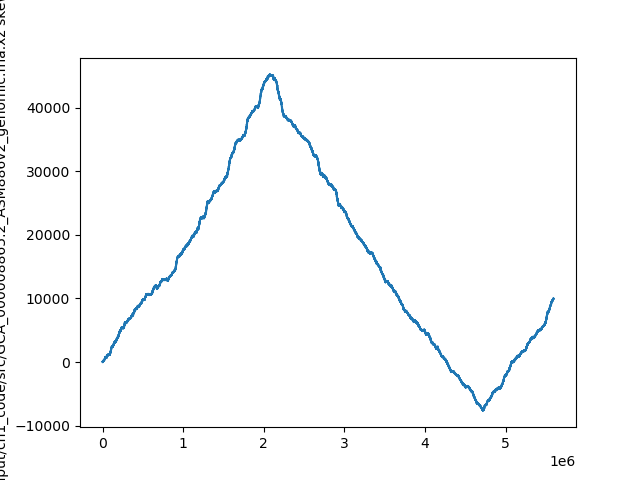
Min position (ori): 4719166
Max position (ter): 2073768
⚠️NOTE️️️⚠️
The material talks about how not all bacteria have a single peak and single valley. Some may have multiple. The reasoning for this still hasn't been discovered. It was speculated at one point that some bacteria may have multiple ori / ter regions.
↩PREREQUISITES↩
Within the ori region, there exists several copies of some k-mer pattern. These copies are referred to as DnaA boxes.

The DnaA protein binds to a DnaA box to activate the process of DNA replication. Through experiments, biologists have determined that DnaA boxes are typical 9-mers. The 9-mers may not match exactly -- the DnaA protein may bind to ...
⚠️NOTE️️️⚠️
The reason why multiple copies of the DnaA box exist probably has to do with DNA mutation. If one of the copies mutates to a point where the DnaA protein no longer binds to it, it can still bind to the other copies.
In the example below, the general vicinity of E. coli's ori is found using GC skew, then that general vicinity is searched for repeating 9-mers. These repeating 9-mers are potential DnaA box candidates.
Calculating skew for: ...
Result: [0, 0, 1, 0,...
Ori vicinity (min pos): 4719166
In the ori vicinity, found clusters of k=9 (at least 3 occurrences in window of 500) in ... at...
A transcription factor / regulatory protein is an enzyme that influences the rate of gene expression for some set of genes. As the saturation of a transcription factor changes, so does the rate of gene expression for the set of genes that it influences.
Transcription factors bind to DNA near the genes they influence: a transcription factor binding site is located in a gene's upstream region and the sequence at that location is a fuzzy nucleotide sequence of length 8 to 12 called a regulatory motif. The simplest way to think of a regulatory motif is a regex pattern without quantifiers. For example, the regex [AT]TT[GC]CCCTA may match to ATTGCCCTA, ATTCCCCTA, TTTGCCCTA, and TTTCCCCTA. The regex itself is the motif, while the sequences being matched are motif members.

The production of transcription factors may be tied to certain internal or external conditions. For example, imagine a flower where the petals...
The external conditions of sunlight and temperature causes the saturation of some transcription factors to change. Those transcription factors influence the rate of gene expression for the genes that control the bunching and spreading of the petals.

↩PREREQUISITES↩
Given an organism, it's suspected that some physical change in that organism is linked to a transcription factor. However, it isn't known ...
A special device is used to take snapshots of the organism's mRNA at different points in time: DNA microarray / RNA sequencer. Specifically, two snapshots are taken:
Comparing these snapshots identifies which genes have noticeably differing rates of gene expression. If these genes (or a subset of these genes) were influenced by the same transcription factor, their upstream regions would contain members of that transcription factor's regulatory motif.
Since neither the transcription factor nor its regulatory motif are known, there is no specific motif to search for in the upstream regions. But, because motif members are typically similar to each other, motif matrix finding algorithms can be used on these upstream regions to find sets of similar k-mers. These similar k-mers may all be members of the same transcription factor's regulatory motif.

In the example below, a set of genes in baker's yeast (Saccharomyces cerevisiae) are suspected of being influenced by the same transcription factor. These genes are searched for a common motif. Assuming one is found, it could be the motif of the suspected transcription factor.
⚠️NOTE️️️⚠️
The example below hard codes k to 18, but you typically don't know what k should be set to beforehand. The Pevzner book doesn't discuss how to work around this problem. A strategy for finding k may be to run the motif matrix finding algorithm multiple times, but with a different k each time. For each member, if the k-mers selected across the runs came from the same general vicinity of the gene's upstream region, those k-mers may either be picking ...
Organism is baker's yeast. Suspected genes influenced by transcription factor: THI12, YHL017W, SYN8, YCG1, UBX5, and KEI1.
Searching for 18-mer across a set of 6 gene upstream regions...
GAAAAGAAAGAAAAAGGA
GAAAAGAAAAAGAAAAAA
GAAAGAAAAAGAAAAAAA
AAAAGGAAAAAAAGAAGA
GAAATGAAAAGGAACAGT
AAAATCAAAAAAATAAAT
Score is: 22
A peptide is a miniature protein consisting of a chain of amino acids anywhere between 2 to 100 amino acids in length.

Most peptides are synthesized through the central dogma of molecular biology: a segment of the DNA that encodes the peptide is transcribed to mRNA, which in turn is translated to a peptide by a ribosome.
Non-ribosomal peptides (NRP) however, aren't synthesized via the central dogma of molecular biology. Instead, giant proteins typically found in bacteria and fungi called NRP synthetase build out these peptides by growing them one amino acid at a time.
Each segment of an NRP synthetase protein responsible for the outputting a single amino acid is called an adenylation domain. The example above has 5 adenylation domains, each of which is responsible for outputting a single amino acid of the peptide it produces.
NRPs may be cyclic. Common use-cases for NRPs:
⚠️NOTE️️️⚠️
According to the Wikipedia article on NRPs, there exist a wide range of peptides that are not synthesized by ribosomes but the term non-ribosomal peptide typically refers to the ones synthesized by NRP synthetases.
↩PREREQUISITES↩
Unlike ribosomal peptides, NRPs aren't encoded in the organism's DNA. As such, their sequence can't be inferred by directly by looking through the organism's DNA sequence.
Instead, a sample of the NRP needs to be isolated and passed through a mass spectrometer. A mass spectrometer is a device that shatters and bins molecules by their mass-to-charge ratio: Given a sample of molecules, the device randomly shatters each molecule in the sample (forming ions), then bins each ion by its mass-to-charge ratio ().
The output of a mass spectrometer is a plot called a spectrum. The plot's ...
For example, given a sample containing multiple instances of the linear peptide NQY, the mass spectrometer will take each instance of NQY and randomly break the bonds between its amino acids:
Each subpeptide then will have its mass-to-charge ratio measured, which in turn gets converted to a set of potential masses by performing basic math. With these potential masses, it's possible to infer which amino acids make up the peptide as well as the peptide sequence.
In the example below, peptide sequences are inferred from a noisy spectrum for the cyclopeptide Viomycin. The elements of each inferred peptide sequence are amino acid masses rather than the amino acids themselves (e.g. instead of S being output at a position, the mass of S is output -- 87). Since the spectrum is noisy, the inferred peptide sequences are also noisy (e.g. instead of an amino acid mass 87 showing up as exactly 87 in the peptide sequence, it may show up as 87.2, 86.9, etc...).
Note that the correct peptide sequence isn't guaranteed to be inferred. Also, since Viomycin is a cyclopeptide, the correct peptide may be inferred in a wrapped form (e.g. the cyclopeptide 128-113-57 may show up as 128-113-57, 113-57-128, or 57-128-113).
⚠️NOTE️️️⚠️
I artificially generated a spectrum for Viomycin from the sequence listed on KEGG.
Sequence 0 beta-Lys 1 Dpr 2 Ser 3 Ser 4 Ala 5 Cpd (Cyclization: 1-5)
Gene 0 vioO [UP:Q6WZ98] vioM [UP:Q6WZA0]; 1 vioF [UP:Q6WZA7]; 2-3 vioA [UP:Q6WZB2]; 4 vioI [UP:Q6WZA4]; 5 vioG [UP:Q84CG4]
Organism Streptomyces vinaceus
Type NRP
The problem is that I have no idea what the 5th amino acid is: Cpd (I arbitrarily put it's mass as 200) and I'm unsure of the mapping I found for Dpr (2,3-diaminopropionic acid has mass of 104). The peptide sequence being searched for in the example below is 128-104-87-87-71-200.
Given the ...
Top 24 captured mino acid masses (rounded to 1): [86.8, 86.9, 87.0, 87.1, 71.1, 71.2, 70.9, 71.0, 128.3, 199.8, 199.9, 200.0, 200.1, 103.7, 103.9, 104.0, 104.1, 127.9, 128.0]
For peptides between 673.1 and 680.9...
Genome rearrangement is form of mutation where chromosomes go through structural changes. These structural changes include chromosome segments getting ...
shuffled into a different order (translocation, fission, fusion) or direction (reversal).
For example, a segment of chromosome breaks off and rejoins, but each end of that segment joins back up at a different point.


deleted.
For example, a segment of a chromosome breaks off and DNA repair mechanisms close the gap.

duplicated.
For example, a segment of a chromosome breaks off and DNA repair mechanisms close the gap, but that broken off segment may still re-attach at a different location.

There are fragile regions of chromosomes where breakages are more likely to occur. For example, the ABL-BCR fusion protein, a protein implicated in the development of a cancer known as chronic myeloid leukemia, is the result of human chromosomes 9 and 22 breaking and fusing back together in a different order: Chromosome 9 contains the gene for ABL while chromosome 22 contains the gene for BCR and both genes are in fragile regions of their respective chromosome. If those fragile chromosome regions both break but fuse back together in the wrong order, the ABL-BCR chimeric gene is formed.
As shown with the ABL-BCR fusion protein example above, genome rearrangements often result in the sterility or death of the organism. However, when a species branches off from an existing one, genome rearrangements are likely responsible for at least some of the divergence. That is, the two related genomes will share long stretches of similar genes, but these long stretches will appear as if they had been randomly cut-and-paste and / or randomly reversed when compared to the other. For example, humans and mice have a shared ancestry and as such share a vast number of long stretches (around 280).
These long stretches of similar genes are called synteny blocks. For example, the following genome rearrangement mutations result in 4 synteny blocks shared between the two genomes ...
[G1, G2][G3][G4, G5, G6] (although they're reversed)[G7, G8, G9]↩PREREQUISITES↩
Synteny blocks are identified by first finding matching k-mers and reverse complement matching k-mers, then combining matches that are close together (clustering) to reveal the long stretches of matches that make up synteny blocks.
The visual manifestation of this concept is the genomic dot-plot and synteny graph. A genomic dot-plot is a 2D plot where each axis is assigned to one of the genomes and a dot is placed at each coordinate containing a match, while a synteny graph is the clustered form of a genomic dot-plot that reveals synteny blocks.

The synteny graph above reveals that 4 synteny blocks are shared between the genomes. One of the synteny blocks is a normal match (C) while three are matching against their reverse complements (A, B, and D).

In the example below, two species of the Mycoplasma bacteria are analyzed to find the synteny blocks between them. The output reveals that pretty much the entirety of both genomes are shared, just in a different order.
Finding synteny blocks for...
NOTE: Nucleotide codes that aren't ACGT get filtered out of the genomes.
Generating genomic dotplot...
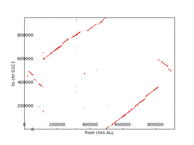
Clustering genomic dotplot to snyteny graph...
Generating synteny graph...
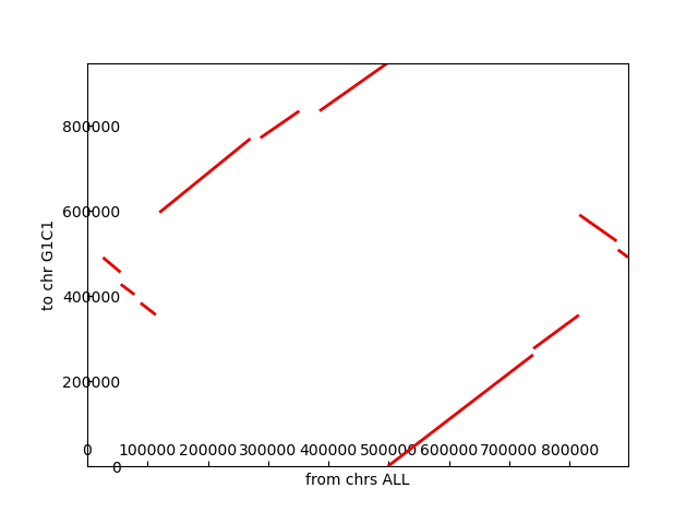
Mapping synteny graph matches to IDs using x-axis genome...
↩PREREQUISITES↩
A reversal is the most common type of genome rearrangement mutation: A segment of chromosome breaks off and ends up re-attaching, but with the ends swapped.

The theory is that genome rearrangements between two species take the parsimonious path (or close to it). Since reversals are the most common form of genome rearrangement mutation, by calculating a parsimonious reversal path (smallest set of reversals) it's possible to get an idea of how the two species branched off.
Note that there may be many parsimonious reversal paths between two genomes with shared synteny blocks.

Given a parsimonious reversal path, it may be that one of the genomes in the reversal path is the parent species (or close to it).

In the example below, two species of the Mycoplasma bacteria are analyzed to find a parsimonious reversal path using the breakpoint graph algorithm. The output reveals that only 1 reversal is responsible for the change in species. As such, it's very likely that one species broke off from the other rather than there being a shared parent species.
Solving a parsimonious reversal path for...
NOTE: Nucleotide codes that aren't ACGT get filtered out of the genomes.
Generating genomic dotplot...
Clustering genomic dotplot to snyteny graph...
Generating synteny graph...
Mapping synteny graph matches to IDs using x-axis genome...
Generating permutations for genomes...
Generating reversal path on genomes that are cyclic=True...
INITIAL red_p_list=[['+G2C1_B0', '+G2C1_B1', '+G2C1_B2', '-G2C1_B7', '-G2C1_B6', '-G2C1_B5', '-G2C1_B4', '-G2C1_B3', '+G2C1_B8', '+G2C1_B9']]

red_p_list=[['+G2C1_B0', '+G2C1_B1', '+G2C1_B2', '+G2C1_B3', '+G2C1_B4', '+G2C1_B5', '+G2C1_B6', '+G2C1_B7', '+G2C1_B8', '+G2C1_B9']]

When scientists work with biological entities, those entities are either present day entities or relics of extinct entities (paleontology). In certain cases, it's reasonable to assume the shared ancestry of a set of present day entities by comparing their features to those of extinct relics. For example, ...

In most cases however, there are no relics. For example, extinct viruses or bacteria typically don't leave much evidence around in the same way that ...
In such cases, it's still possible to infer the evolutionary history of a set of present day species by comparing their features to see how diverged they are. Those features could be phenotypic features (e.g. behavioural or physical features) or molecular features (e.g. DNA sequences, protein sequences, organelles and other cell features).
The process of inferring evolutionary history by comparing features for divergence is called phylogeny. Phylogeny algorithms provide insight into ...

Oftentimes, phylogeny produces much more accurate results than simply eye-balling it (as was done in the initial example), but ultimately the quality of the result is dependent on what features are being measured and the metric used for measurement. Prior to sequencing technology, most phylogeny was done by comparing phenotypic features (e.g. character tables). Common practice now is to use molecular features (e.g. DNA sequencing) since those have more information that's definitive and less biased (e.g. phenotypic features are subject to human interpretation).
↩PREREQUISITES↩
Evolutionary history is often displayed as a tree called a phylogenetic tree, where leaf nodes represent known entities and internal nodes represent inferred ancestor entities. Depending on the phylogeny algorithm used, the tree may be either a rooted tree or an unrooted tree. The difference is that a rooted tree infers parent-child relationships of ancestors while an unrooted tree does not.

In the example above, the rooted tree (left diagram) shows ancestors B and C as branching off (evolving) from their common ancestor A. The unrooted tree (right diagram) shows ancestors B and C but doesn't provide infer which branched off the other. It could be that ancestor B ultimately descended from C or vice versa.
SARS-CoV-2 is the virus that causes COVID-19. The example below measures SARS-CoV-2 spike protein sequences collected from different patients to produce its evolutionary history. The metric used to measure how diverged two sequences are from each other is global alignment using a BLOSUM80 scoring matrix. Once divergences (distances) are calculated, the neighbour joining phylogeny algorithm is used to generate a phylogenetic tree.
⚠️NOTE️️️⚠️
BLOSUM80 was chosen because SARS-CoV-2 is a relatively new virus (~2 years). I don't know if it was a good choice because I've been told viruses mutate more rapidly, so maybe BLOSUM62 would have been a better choice.
The original NCBI dataset had 30k to 40k unique spike sequences. I couldn't justify sticking all of that into the git repo (too large) so I whittled it down to a random sample of 1000.
From that 1000, only a small sample are selected to run the code. The problem is that sequence alignments are computationally expensive and Python is slow. Doing a sequence alignment between two spike protein sequences on my VM takes a long time (~4 seconds per alignment), so for the full 1000 sequences the total running time would end up being ~4 years (if I calculated it correctly - single core).
Given a random sample of 6 sequences from 1000_unique_sarscov2_spike_seqs.json.xz and the following alignment weights...
A R N D C Q E G H I L K M F P S T W Y V B J Z X *
A 5 -2 -2 -2 -1 -1 -1 0 -2 -2 -2 -1 -1 -3 -1 1 0 -3 -2 0 -2 -2 -1 -1 -6
R -2 6 -1 -2 -4 1 -1 -3 0 -3 -3 2 -2 -4 -2 -1 -1 -4 -3 -3 -1 -3 0 -1 -6
N -2 -1 6 1 -3 0 -1 -1 0 -4 -4 0 -3 -4 -3 0 0 -4 -3 -4 5 -4 0 -1 -6
D -2 -2 1 6 -4 -1 1 -2 -2 -4 -5 -1 -4 -4 -2 -1 -1 -6 -4 -4 5 -5 1 -1 -6
C -1 -4 -3 -4 9 -4 -5 -4 -4 -2 -2 -4 -2 -3 -4 -2 -1 -3 -3 -1 -4 -2 -4 -1 -6
Q -1 1 0 -1 -4 6 2 -2 1 -3 -3 1 0 -4 -2 0 -1 -3 -2 -3 0 -3 4 -1 -6
E -1 -1 -1 1 -5 2 6 -3 0 -4 -4 1 -2 -4 -2 0 -1 -4 -3 -3 1 -4 5 -1 -6
G 0 -3 -1 -2 -4 -2 -3 6 -3 -5 -4 -2 -4 -4 -3 -1 -2 -4 -4 -4 -1 -5 -3 -1 -6
H -2 0 0 -2 -4 1 0 -3 8 -4 -3 -1 -2 -2 -3 -1 -2 -3 2 -4 -1 -4 0 -1 -6
I -2 -3 -4 -4 -2 -3 -4 -5 -4 5 1 -3 1 -1 -4 -3 -1 -3 -2 3 -4 3 -4 -1 -6
L -2 -3 -4 -5 -2 -3 -4 -4 -3 1 4 -3 2 0 -3 -3 -2 -2 -2 1 -4 3 -3 -1 -6
K -1 2 0 -1 -4 1 1 -2 -1 -3 -3 5 -2 -4 -1 -1 -1 -4 -3 -3 -1 -3 1 -1 -6
M -1 -2 -3 -4 -2 0 -2 -4 -2 1 2 -2 6 0 -3 -2 -1 -2 -2 1 -3 2 -1 -1 -6
F -3 -4 -4 -4 -3 -4 -4 -4 -2 -1 0 -4 0 6 -4 -3 -2 0 3 -1 -4 0 -4 -1 -6
P -1 -2 -3 -2 -4 -2 -2 -3 -3 -4 -3 -1 -3 -4 8 -1 -2 -5 -4 -3 -2 -4 -2 -1 -6
S 1 -1 0 -1 -2 0 0 -1 -1 -3 -3 -1 -2 -3 -1 5 1 -4 -2 -2 0 -3 0 -1 -6
T 0 -1 0 -1 -1 -1 -1 -2 -2 -1 -2 -1 -1 -2 -2 1 5 -4 -2 0 -1 -1 -1 -1 -6
W -3 -4 -4 -6 -3 -3 -4 -4 -3 -3 -2 -4 -2 0 -5 -4 -4 11 2 -3 -5 -3 -3 -1 -6
Y -2 -3 -3 -4 -3 -2 -3 -4 2 -2 -2 -3 -2 3 -4 -2 -2 2 7 -2 -3 -2 -3 -1 -6
V 0 -3 -4 -4 -1 -3 -3 -4 -4 3 1 -3 1 -1 -3 -2 0 -3 -2 4 -4 2 -3 -1 -6
B -2 -1 5 5 -4 0 1 -1 -1 -4 -4 -1 -3 -4 -2 0 -1 -5 -3 -4 5 -4 0 -1 -6
J -2 -3 -4 -5 -2 -3 -4 -5 -4 3 3 -3 2 0 -4 -3 -1 -3 -2 2 -4 3 -3 -1 -6
Z -1 0 0 1 -4 4 5 -3 0 -4 -3 1 -1 -4 -2 0 -1 -3 -3 -3 0 -3 5 -1 -6
X -1 -1 -1 -1 -1 -1 -1 -1 -1 -1 -1 -1 -1 -1 -1 -1 -1 -1 -1 -1 -1 -1 -1 -1 -6
* -6 -6 -6 -6 -6 -6 -6 -6 -6 -6 -6 -6 -6 -6 -6 -6 -6 -6 -6 -6 -6 -6 -6 -6 1
The tree generated by neighbour joining phylogeny is (distances measured using global alignment, edge lengths scaled to 0.1) ...

↩PREREQUISITES↩
An unknown ancestor's features are probabilistically inferrable via the features of entities that descend from it.

The example above infers phenotypic features for the common ancestor of leopard and tiger. If a feature is present and the same in both, it's safe to assume that it was present in their common ancestor as well (e.g. 4 legs). Otherwise, there's still some smaller chance that the feature was present, possibly with some variability in how it manifested (e.g. type of coat pattern).
With the advent of sequencing technology, the practice of using phenotypic features for phylogeny was superseded by sequencing data. When sequences are used, the features are the sequences themselves, meaning that the sequence of the common ancestor is what gets inferred.

The example below infers the spike protein sequences for the ancestors of SARS-CoV-2 variants. First, a phylogenetic tree is generated using BLOSUM80 as the distance metric. Then, the sequences are all aligned together using BLOSUM80 (multiple alignment, not pairwise alignment as was used for the distance metric). The sequences of ancestors are inferred using those aligned sequences.
⚠️NOTE️️️⚠️
This is badly cobbled together code. It's taking the code from the previous section's example and embedding/duct-taping even more pieces from the sequence alignment module just to get a running example. In a perfect world I would just import the sequence alignment module, but that module lives in a separate container. This is the best I can do.
Running this is even slower than the previous section's example, so the sample size has been reduced even further.
Given a random sample of 3 sequences from 1000_unique_sarscov2_spike_seqs.json.xz and the following alignment weights...
A R N D C Q E G H I L K M F P S T W Y V B J Z X
A 5 -2 -2 -2 -1 -1 -1 0 -2 -2 -2 -1 -1 -3 -1 1 0 -3 -2 0 -2 -2 -1 -1
R -2 6 -1 -2 -4 1 -1 -3 0 -3 -3 2 -2 -4 -2 -1 -1 -4 -3 -3 -1 -3 0 -1
N -2 -1 6 1 -3 0 -1 -1 0 -4 -4 0 -3 -4 -3 0 0 -4 -3 -4 5 -4 0 -1
D -2 -2 1 6 -4 -1 1 -2 -2 -4 -5 -1 -4 -4 -2 -1 -1 -6 -4 -4 5 -5 1 -1
C -1 -4 -3 -4 9 -4 -5 -4 -4 -2 -2 -4 -2 -3 -4 -2 -1 -3 -3 -1 -4 -2 -4 -1
Q -1 1 0 -1 -4 6 2 -2 1 -3 -3 1 0 -4 -2 0 -1 -3 -2 -3 0 -3 4 -1
E -1 -1 -1 1 -5 2 6 -3 0 -4 -4 1 -2 -4 -2 0 -1 -4 -3 -3 1 -4 5 -1
G 0 -3 -1 -2 -4 -2 -3 6 -3 -5 -4 -2 -4 -4 -3 -1 -2 -4 -4 -4 -1 -5 -3 -1
H -2 0 0 -2 -4 1 0 -3 8 -4 -3 -1 -2 -2 -3 -1 -2 -3 2 -4 -1 -4 0 -1
I -2 -3 -4 -4 -2 -3 -4 -5 -4 5 1 -3 1 -1 -4 -3 -1 -3 -2 3 -4 3 -4 -1
L -2 -3 -4 -5 -2 -3 -4 -4 -3 1 4 -3 2 0 -3 -3 -2 -2 -2 1 -4 3 -3 -1
K -1 2 0 -1 -4 1 1 -2 -1 -3 -3 5 -2 -4 -1 -1 -1 -4 -3 -3 -1 -3 1 -1
M -1 -2 -3 -4 -2 0 -2 -4 -2 1 2 -2 6 0 -3 -2 -1 -2 -2 1 -3 2 -1 -1
F -3 -4 -4 -4 -3 -4 -4 -4 -2 -1 0 -4 0 6 -4 -3 -2 0 3 -1 -4 0 -4 -1
P -1 -2 -3 -2 -4 -2 -2 -3 -3 -4 -3 -1 -3 -4 8 -1 -2 -5 -4 -3 -2 -4 -2 -1
S 1 -1 0 -1 -2 0 0 -1 -1 -3 -3 -1 -2 -3 -1 5 1 -4 -2 -2 0 -3 0 -1
T 0 -1 0 -1 -1 -1 -1 -2 -2 -1 -2 -1 -1 -2 -2 1 5 -4 -2 0 -1 -1 -1 -1
W -3 -4 -4 -6 -3 -3 -4 -4 -3 -3 -2 -4 -2 0 -5 -4 -4 11 2 -3 -5 -3 -3 -1
Y -2 -3 -3 -4 -3 -2 -3 -4 2 -2 -2 -3 -2 3 -4 -2 -2 2 7 -2 -3 -2 -3 -1
V 0 -3 -4 -4 -1 -3 -3 -4 -4 3 1 -3 1 -1 -3 -2 0 -3 -2 4 -4 2 -3 -1
B -2 -1 5 5 -4 0 1 -1 -1 -4 -4 -1 -3 -4 -2 0 -1 -5 -3 -4 5 -4 0 -1
J -2 -3 -4 -5 -2 -3 -4 -5 -4 3 3 -3 2 0 -4 -3 -1 -3 -2 2 -4 3 -3 -1
Z -1 0 0 1 -4 4 5 -3 0 -4 -3 1 -1 -4 -2 0 -1 -3 -3 -3 0 -3 5 -1
X -1 -1 -1 -1 -1 -1 -1 -1 -1 -1 -1 -1 -1 -1 -1 -1 -1 -1 -1 -1 -1 -1 -1 -1
INDEL=-6.0
The tree generated by neighbour joining phylogeny ALONG WITH INFERRED ANCESTRAL SEQUENCES is (distances measured using global alignment, edge lengths scaled to 0.1) ...

Gene expression is the biological process by which a gene (segment of DNA) is synthesized into a gene product (e.g. protein).
As an organism changes state, its gene expression levels change as well. For example, when a bacteria's flagella initially starts moving, a gene may have either an ...
The subset of genes whose gene expression either increase or decrease are somehow linked to initial flagella movement. It could be that a linked gene is either responsible for a byproduct of the flagella movement.

The same idea extends to diseases and treatments. For example, a cancerous human blood cell may have a subset of genes where gene expression is vastly different from its non-cancerous counterpart. Identifying the genes linked to human blood cancer could lead to ...
The common way to measure gene expression is to inspect the RNA within a cell. A snapshot of all RNA transcripts within a cell at a given point in time, called a transcriptome, can be captured using RNA sequencing technology. Both the RNA sequences and the counts of those transcripts (number of instances) are captured. Given that an RNA transcript is simply a transcribed "copy" of the DNA it came from (it identifies the gene), a snapshot indirectly shows the amount of gene expression taking place for each gene at the time that snapshot was taken.
Differential gene expression analysis is the process of capturing and comparing multiple RNA snapshots for an organism in different states. The comparisons help identify which genes are influenced by / responsible for the relevant state changes.
There are two broad categories of differential gene expression analysis: time-course and conditional. For some population, ...
time-course captures RNA snapshots at different points (e.g. apply drug to culture of cancerous blood cells, then measure gene expression levels once per hour).
| hour 0 | hour 1 | hour 2 | ... | |
|---|---|---|---|---|
| Gene A | 100 | 100 | 100 | ... |
| Gene B | 100 | 70 | 50 | ... |
| Gene C | 100 | 110 | 140 | ... |
| ... | ... | ... | ... | ... |
conditional captures RNA snapshots across different conditions (e.g. compare gene expression levels across 50 blood cancer patients vs 50 cancer-free patients).
| patient1 (cancer) | patient2 (cancer) | patient3 (non-cancer) | ... | |
|---|---|---|---|---|
| Gene X | 100 | 100 | 100 | ... |
| Gene Y | 100 | 110 | 50 | ... |
| Gene Z | 100 | 110 | 140 | ... |
| ... | ... | ... | ... | ... |
⚠️NOTE️️️⚠️
The sub-section describes how to deal with time-courses. There is no sub-section describing how to deal with conditionals. The Pevzner book never went over it. But, the final challenge question did throw a conditional dataset at you and asked you to solve some problem. It seems that for conditional datasets, the key thing you need to do is filter out unrelated genes before doing anything. For the challenge in the Pevzner book, I simply compared a gene's average gene expression between cancer vs non-cancer to determine if it was relevant (if the offset was large enough, I decided it was relevant).
↩PREREQUISITES↩
A time-course experiment captures RNA snapshots at different points in time. For example, a biologist infects a cell culture with a pathogen, then measures gene expression levels within that culture every hour.
| hour 0 | hour 1 | hour 2 | hour 3 | hour 4 | |
|---|---|---|---|---|---|
| Gene X | 100 | 100 | 50 | 50 | 20 |
| Gene Y | 20 | 50 | 50 | 100 | 100 |
| Gene Z | 50 | 50 | 50 | 50 | 50 |
| ... | ... | ... | ... | ... | ... |
If two genes have similar gene expression vectors, it could be that they're related in some way (e.g. regulated by the same transcription factor). Clustering a set of genes by their gene expression vectors helps identify these relationships. If done properly, genes within the same cluster should have gene expression vectors that are more similar to each other than to those in other clusters (good clustering principle).
Gene clusters can then be passed off to a biologist for further investigation (e.g. to confirm if they're actually influenced by the same transcription factor).
The example below clusters a time-course for astrocyte cells infected with H5N1 bird flu. The time-course measures gene expression at 6, 12, and 24 hours into infection. The clustering process builds a phylogenetic tree, where a simple heuristic determines parts of the tree that represent clusters (e.g. regions of interest).
⚠️NOTE️️️⚠️
This dataset is from the NCBI gene expression omnibus (GEO): Influenza virus H5N1 infection of U251 astrocyte cell line: time course. You may be able to use other datasets from the GEO with this same code -- use the GDS browser if you want to find more.
GDS6010
Title: Influenza virus H5N1 infection of U251 astrocyte cell line: time course
Summary: Analysis of U251 astrocyte cells infected with the influenza H5N1 virus for up to 24 hours. Results provide insight into the immune response of astrocytes to H5N1 infection.
Organism: Homo sapiens
Platform: GPL6480: Agilent-014850 Whole Human Genome Microarray 4x44K G4112F (Probe Name version)
Citation: Lin X, Wang R, Zhang J, Sun X et al. Insights into Human Astrocyte Response to H5N1 Infection by Microarray Analysis. Viruses 2015 May 22;7(5):2618-40. PMID: 26008703
Reference Series: GSE66597
Sample count: 18
Value type: transformed count
Series published: 2016/01/04
There are too many genes here for the clustering algorithm (Python is slow). As such, standard deviation is used to filter out gene expression vectors that don't dramatically change during the time-course. The experiment did come with a control group: a second population of the same cell line but uninfected. Maybe instead of standard deviation, a better filtering approach would be to only include genes whose gene expression pattern is vastly different between control group vs experimental group.
The original data set was too large. I removed the replicates and only kept hour 24 of the control group.
Executing neighbour joining phylogeny soft clustering using the following settings...
{
filename: GDS6010.soft_no_replicates_single_control.xz,
gene_column: ID_REF, # col name for gene ID
sample_columns: [
GSM1626001, # col name for control @ 24 hrs (treat this as a measure of "before infection")
GSM1626004, # col name for infection @ 6 hrs
GSM1626007, # col name for infection @ 12 hrs
GSM1626010 # col name for infection @ 24 hrs
],
std_dev_limit: 1.6, # reject anything with std dev less than this
metric: euclidean, # OPTIONS: euclidean, manhattan, cosine, pearson
dist_capture: 0.5,
edge_scale: 3.0
}
The following neighbour joining phylogeny tree was produced ...

The following clusters were estimated ...
A point mutation is a mutation where a specific location of a DNA sequence has its nucleotide substituted for another (e.g. a C got mutated to a G). Across a population, if a specific point mutation occurs frequently enough, it's considered a single nucleotide polymorphism (SNP) rather than a mutation (a common variation of some species's genome). Specifically, if the frequency of the substitution occurring is ...
Studies commonly attempt to associate SNPs with diseases. By comparing SNPs between a diseased population vs non-diseased population, scientists are able to discover which SNPs are responsible for a disease / increase the risk of a disease occurring. For example, a study might find that the population of heart attack victims had a location with a higher likelihood of G vs C.
↩PREREQUISITES↩
The SNPs / point mutations that an individual organism has are identified through a process called read mapping. Read mapping attempts to align the individual organism's sequenced DNA segments (e.g. reads, read-pairs, contigs) to an idealized genome for the population that organism belongs to (e.g. species, race, etc..), called a reference genome. The result of the alignment should have few indels and a fair amount of mismatches, where those mismatches identify that organism's SNPs / point mutations.
Since read mapping for SNP / point mutation identification focuses on identifying mismatches and not indels, traditional sequence alignment algorithms aren't required. More efficient substring finding algorithms can be used instead. Specifically, if you have a substring that you're trying to find in a sequence, and you know it can tolerate d mismatches at most, separate it into d + 1 blocks. It's impossible for d mismatches to exist across d + 1 blocks. There are more blocks than there are mismatches -- at least one of the blocks must match exactly.
These blocks are called seeds, and the act of finding seeds and testing the hamming distance of the extended region is called seed extension.
The example below read maps the reads from a Mycoplasma agalactiae genome to a reference genome for Mycoplasma bovis.
Executing checkpointed BWT search algorithm using the following settings (reverse complements of reads automatically included)...
reference_genome_filename: Mycoplasma bovis - GCA_000696015.1_ASM69601v1_genomic.fna.xz
reads_filename: Mycoplasma agalactiae - READS.txt.xz
max_mismatch: 2
pad_marker: _
end_marker: $
last_tallies_checkpoint_n: 20
first_indexes_checkpoint_n: 20
CP005933.1 Mycoplasma bovis CQ-W70, complete genome
CPU optimized C++ global alignment - Simple global alignment is C++ with all optimizations turned on AND multi-threading or fibers that optimize work size to fit in cache lines.
GPU optimized C++ global alignment - Simple global alignment in Nvidia's HPC SDK C++ where GPU "thread" is optimized to fit in caches. Maybe do the divide-and-conquer variant as well. (divide and conquer might be a good idea because it'll work on super fat sequences)
GPU optimized C++ probabilistic multiple alignment - Probabilistic multiple alignment in Nvidia's HPC SDK C++ where GPU "thread" is optimized to fit in caches.
Deep-learning Regulatory Motif Detection - Try training a deep learning model to "find" regulatory motifs for new transcription factors based on past training data.
Global alignment that takes genome rearrangements into account - multiple chromosomes, chromosomes becoming circular or linear, reversals, fissions, fusions, copies, etc..
Organism lookup by k-mer - Two-tiered database containing k-mers. The first tier is an "inverse index" of k-mers that rarely appear across all organisms (unique or almost unique to the genome) exposed as either a trie / hashtable (for exact lookups) or possibly as a list where highly optimized miniature alignments get performed (for fuzzy lookups -- SIMD + things fit nicely into cache lines). It widdles down the list of organism for the second tier, which is a full on database search for each matches across all k-mers.
K-mer hierarchical clustering - Hierarchical cluster together similar k-mers using either pearson similarity/pearson distance [between one/zero vector of sub-k-mers] or sequence alignment distance to form its distance matrix / similarity matrix. This is useful for when you're trying to identify which organism a sequence belongs to by searching for its k-mers in a database. The k-mers that make up the database would be clustered, and k-mers that closely cluster together under a branch of the hierarchical cluster tree are those you'd be more cautious with -- the k-mer may have matched but it could have actually been a corrupted form of one of the other k-mers in the cluster (sequencing error).
This logic also applies to spell checking. Words that cluster together closely are more likely to be mis-identified by a standard spellchecker, meaning individual clusters should have their own spell checking strategies? If you're going to do this with words, use a factor in QWERTY keyboard key distances into the similarity / distance matrix.
Hierarchical clustering explorer - Generate a neighbour joining phylogeny tree based on pearson distance of sequence alignment distance, then visualize the tree and provide the user with "interesting" internal nodes (clusters). In this case, "interesting" would be any internal node where the distance to most leaf nodes is within some threshold / average / variance / etc... Also, maybe provide an "idealized" view of the clustered data for each internal node (e.g. average the vectors for the leaves to produce the vector for the internal node).
Another idea is to take the generated tree and convert it back into distance matrix. If the data isn't junk, the distance metric isn't junk, and the data is clusterable on that distance metric, the generated distance matrix should match closely to the input distance metric. The tool can warn the user if it doesn't.
Soft hierarchical clustering - Build out a neighbour joining phylogeny tree. Each internal node is a cluster. The distance between that internal node to all leaf nodes can be used to define the probability that the leaf node belongs to that cluster? This makes sense because neighbour joining phylogeny produces unrooted trees (simple trees). If it were a rooted tree, you could say that internal node X leaf nodes A, B, and C -- meaning that A, B and C are members of cluster X. But, because it's unrooted, technically any leaf node in the graph could be a member of cluster X.
This relates to the idea above (hierarchical clustering explorer) -- You can identify "interesting clusters" using this (e.g. a small group tightly clustered together) and return it to the user for inspection.
Hierarchical clustering as a means of detecting outliers - Cluster data using neighbouring join phylogeny. How far is each leaf node to its parent internal node? Find any that are grossly over the average / squared error distortion / some other metric? Report it. Try other ways as well (e.g. pick a root and see how far it is from the root -- root picked using some metric like avg distance between leaf nodes / 2 or squared error distortion).
This relates to the idea above (soft hierarchical clustering) -- You may be able to identify outliers using soft hierarchical clustering using this (e.g. the probability of being a part of some internal node is way farther than any of the other leaf nodes).
Checkpointed BWT algorithm in C++ - Implement it in modern C++ using concepts, as a generic library
Profile HMMs for protiens that factor in BLOSUM / PAM scoring matrix - Build a basic profile HMM (as discussed in the profile HMM section), but the symbol emission probabilities for the profile HMM should factor in BLOSUM / PAM substitution likelihoods into those symbol emission probabilities. For example, a profile of protein sequences might have a column that contains all As. Even though the other amino acids don't appear in the column (R, N, D, etc..), each will still have a small non-zero probability of symbol emission once those probabilities have been normalized via psuedocounts. This is saying that the those small probabilities should increase / decrease based on something like BLOSUM62. For example, A is much more probable to be replaced by C than it is by W (0 score vs -3 score) -- that should be reflected in the symbol emission porbabilities.
k-mer - A substring of length k within some larger biological sequence (e.g. DNA or amino acid chain). For example, in the DNA sequence GAAATC, the following k-mer's exist:
| k | k-mers |
|---|---|
| 1 | G A A A T C |
| 2 | GA AA AA AT TC |
| 3 | GAA AAA AAT ATC |
| 4 | GAAA AAAT AATC |
| 5 | GAAAT AAATC |
| 6 | GAAATC |
kd-mer - A substring of length 2k + d within some larger biological sequence (e.g. DNA or amino acid chain) where the first k elements and the last k elements are known but the d elements in between isn't known.
When identifying a kd-mer with a specific k and d, the proper syntax is (k, d)-mer. For example, (1, 2)-mer represents a kd-mer with k=1 and d=2. In the DNA sequence GAAATC, the following (1, 2)-mer's exist: G--A, A--T, A--C.
See read-pair.
5' (5 prime) / 3' (3 prime) - 5' (5 prime) and 3' (3 prime) describe the opposite ends of DNA. The chemical structure at each end is what defines if it's 5' or 3' -- each end is guaranteed to be different from the other. The forward direction on DNA is defined as 5' to 3', while the backwards direction is 3' to 5'.
Two complementing DNA strands will always be attached in opposite directions.

DNA polymerase - An enzyme that replicates a strand of DNA. That is, DNA polymerase walks over a single strand of DNA bases (not the strand of base pairs) and generates a strand of complements. Before DNA polymerase can attach itself and start replicating DNA, it requires a primer.

DNA polymerase is unidirectional, meaning that it can only walk a DNA strand in one direction: reverse (3' to 5')
primer - A primer is a short strand of RNA that binds to some larger strand of DNA (single bases, not a strand of base pairs) and allows DNA synthesis to happen. That is, the primer acts as the entry point for special enzymes DNA polymerases. DNA polymerases bind to the primer to get access to the strand.
replication fork - The process of DNA replication requires that DNA's 2 complementing strands be unwound and split open. The area where the DNA starts to split is called the replication fork. In bacteria, the replication fork starts at the replication origin and keeps expanding until it reaches the replication terminus. Special enzymes called DNA polymerases walk over each unwound strand and create complementing strands.
replication origin (ori) - The point in DNA at which replication starts.
replication terminus (ter) - The point in DNA at which replication ends.
forward half-strand / reverse half-strand - Bacteria are known to have a single chromosome of circular / looping DNA. In this DNA, the replication origin (ori) is the region of DNA where replication starts, while the replication terminus (ter) is where replication ends.

If you split up the DNA based on ori and ter being cutting points, you end up with 4 distinct strands. Given that the direction of a strand is 5' to 3', if the direction of the strand starts at...
ori and ends at ter, it's called the forward half-strand.

ter and ends at ori, it's called the reverse half-strand.

⚠️NOTE️️️⚠️
leading half-strand / lagging half-strand - Given the 2 strands that make up a DNA molecule, the strand that goes in the...
This nomenclature has to do with DNA polymerase. Since DNA polymerase can only walk in the reverse direction (3' to 5'), it synthesizes the leading half-strand in one shot. For the lagging half-strand (5' to 3'), multiple DNA polymerases have to used to synthesize DNA, each binding to the lagging strand and walking backwards a small amount to generate a small fragment of DNA (Okazaki fragment). the process is much slower for the lagging half-strand, that's why it's called lagging.
⚠️NOTE️️️⚠️
Okazaki fragment - A small fragment of DNA generated by DNA polymerase for forward half-strands. DNA synthesis for the forward half-strands can only happen in small pieces. As the fork open ups every ~2000 nucleotides, DNA polymerase attaches to the end of the fork on the forward half-strand and walks in reverse to generate that small segment (DNA polymerase can only walk in the reverse direction).
DNA ligase - An enzyme that sews together short segments of DNA called Okazaki fragments by binding the phosphate group on the end of one strand with the deoxyribose group on the other strand.
DnaA box - A sequence in the ori that the DnaA protein (responsible for DNA replication) binds to.
single stranded DNA - A single strand of DNA, not bound to a strand of its reverse complements.

double stranded DNA - Two strands of DNA bound together, where each strand is the reverse complement of the other.

reverse complement - Given double-stranded DNA, each ...
The reverse complement means that a stretch of single-stranded DNA has its direction reversed (5' and 3' switched) and nucleotides complemented.
gene - A segment of DNA that contains the instructions for either a protein or functional RNA.
gene product - The final synthesized material resulting from the instructions that make up a gene. That synthesized material either being a protein or functional RNA.
transcription - The process of transcribing a gene to RNA. Specifically, the enzyme RNA polymerase copies the segment of DNA that makes up that gene to a strand of RNA.

translation - The process of translating mRNA to protein. Specifically, a ribosome takes in the mRNA generated by transcription and outputs the protein that it codes for.

gene expression - The process by which a gene is synthesized into a gene product. When the gene product is...
regulatory gene / regulatory protein - The proteins encoded by these genes affect gene expression for certain other genes. That is, a regulatory protein can cause certain other genes to be expressed more (promote gene expression) or less (repress gene expression).
Regulatory genes are often controlled by external factors (e.g. sunlight, nutrients, temperature, etc..)
feedback loop / negative feedback loop / positive feedback loop - A feedback loop is a system where the output (or some part of the output) is fed back into the system to either promote or repress further outputs.

A positive feedback loop amplifies the output while a negative feedback loop regulates the output. Negative feedback loops in particular are important in biology because they allow organisms to maintain homeostasis / equilibrium (keep a consistent internal state). For example, the system that regulates core temperatures in a human is a negative feedback loop. If a human's core temperature gets too...
In the example above, the output is the core temperature. The body monitors its core temperature and employs mechanisms to bring it back to normal if it goes out of range (e.g. sweat, shiver). The outside temperature is influencing the body's core temperature as well as the internal shivering / sweating mechanisms the body employs.

circadian clock / circadian oscillator - A biological clock that synchronizes roughly around the earth's day-night cycle. This internal clock helps many species regulate their physical and behavioural attributes. For example, hunt during the night vs sleep during the day (e.g. nocturnal owls).
upstream region - The area just before some interval of DNA. Since the direction of DNA is 5' to 3', this area is towards the 5' end (upper end).
downstream region - The area just after some interval of DNA. Since the direction of DNA is 5' to 3', this area is towards the 3' end (lower end).
transcription factor - A regulatory protein that controls the rate of transcription for some gene that it has influence over (the copying of DNA to mRNA). The protein binds to a specific sequence in the gene's upstream region.
motif - A pattern that matches against many different k-mers, where those matched k-mers have some shared biological significance. The pattern matches a fixed k where each position may have alternate forms. The simplest way to think of a motif is a regex pattern without quantifiers. For example, the regex [AT]TT[GC]C may match to ATTGC, ATTCC, TTTGC, and TTTCC.
motif member - A specific nucleotide sequence that matches a motif. For example, given a motif represented by the regex [AT]TT[GC]C, the sequences ATTGC, ATTCC, TTTGC, and TTTCC would be its members.
motif matrix - A set of k-mers stacked on top of each other in a matrix, where the k-mers are either...
For example, the motif [AT]TT[GC]C has the following matrix:
| 0 | 1 | 2 | 3 | 4 |
|---|---|---|---|---|
| A | T | T | G | C |
| A | T | T | C | C |
| T | T | T | G | C |
| T | T | T | C | C |
regulatory motif - The motif of a transcription factor, typically 8 to 12 nucleotides in length.
transcription factor binding site - The physical binding site for a transcription factor. A gene that's regulated by a transcription factor needs a sequence located in its upstream region that the transcription factor can bind to: a motif member of that transcription factor's regulatory motif.
⚠️NOTE️️️⚠️
A gene's upstream region is the 600 to 1000 nucleotides preceding the start of the gene.
complementary DNA (cDNA) - A single strand of DNA generated from mRNA. The enzyme reverse transcriptase scans over the mRNA and creates the complementing single DNA strand.

The mRNA portion breaks off, leaving the single-stranded DNA.

DNA microarray - A device used to compare gene expression. This works by measuring 2 mRNA samples against each other: a control sample and an experimental sample. The samples could be from...
Both mRNA samples are converted to cDNA and are given fluorescent dyes. The control sample gets dyed green while the experimental sample gets dyed red.

A sheet is broken up into multiple regions, where each region has the cDNA for one specific gene from the control sample printed.

The idea is that once the experimental cDNA is introduced to that region, it should bind to the control cDNA that's been printed to form double-stranded DNA. The color emitted in a region should correspond to the amount of gene expression for the gene that region represents. For example, if a region on the sheet is fully yellow, it means that the gene expression for that gene is roughly equal (red mixed with green is yellow).
greedy algorithm - An algorithm that tries to speed things up by taking the locally optimal choice at each step. That is, the algorithm doesn't look more than 1 step ahead.
For example, imagine a chess playing AI that had a strategy of trying to eliminate the other player's most valuable piece at each turn. It would be considered greedy because it only looks 1 move ahead before taking action. Normal chess AIs / players look many moves ahead before taking action. As such, the greedy AI may be fast but it would very likely lose most matches.
Cromwell's rule - When a probability is based on past events, 0.0 and 1.0 shouldn't be used. That is, if you've...
Unless you're dealing with hard logical statements where prior occurrences don't come in to play (e.g. 1+1=2), you should include a small chance that some extremely unlikely event may happen. The example tossed around is "the probability that the sun will not rise tomorrow." Prior recorded observations show that the sun has always risen, but that doesn't mean that there's a 1.0 probability of the sun rising tomorrow (e.g. some extremely unlikely cataclysmic event may prevent the sun from rising).
Laplace's rule of succession - If some independent true/false event occurs n times, and s of those n times were successes, it's natural for people to assume the probability of success is . However, if the number of successes is 0, the probability would be 0.0. Cromwell's rule states that when a probability is based off past events, 0.0 and 1.0 shouldn't be used. As such, a more appropriate / meaningful measure of probability is .
For example, imagine you're sitting on a park bench having lunch. Of the 8 birds you've seen since starting your lunch, all have been pigeons. If you were to calculate the probability that the next bird you'll see a crow, would be flawed because it states that there's no chance that the next bird will be a crow (there obviously is a chance, but it may be a small chance). Instead, applying Laplace's rule allows for the small probability that a crow may be seen next: .
Laplace's rule of succession is more meaningful when the number of trials (n) is small.
pseudocount - When a zero is replaced with a small number to prevent unfair scoring. See Laplace's rule of succession.
randomized algorithm - An algorithm that uses a source of randomness as part of its logic. Randomized algorithms come in two forms: Las Vegas algorithms and Monte Carlo algorithms
Las Vegas algorithm - A randomized algorithm that delivers a guaranteed exact solution. That is, even though the algorithm makes random decisions it is guaranteed to converge on the exact solution to the problem its trying to solve (not an approximate solution).
An example of a Las Vegas algorithm is randomized quicksort (randomness is applied when choosing the pivot).
Monte Carlo algorithm - A randomized algorithm that delivers an approximate solution. Because these algorithms are quick, they're typically run many times. The approximation considered the best out of all runs is the one that gets chosen as the solution.
An example of a Monte Carlo algorithm is a genetic algorithm to optimize the weights of a deep neural network. That is, a step of the optimization requires running n different neural networks to see which gives the best result, then replacing those n networks with n copies of the best performing network where each copy has randomly tweaked weights. At some point the algorithm will stop producing incrementally better results.
Perform the optimization (the entire thing, not just a single step) thousands of times and pick the best network.
consensus string - The k-mer generated by selecting the most abundant column at each index of a motif matrix.
| 0 | 1 | 2 | 3 | 4 | |
|---|---|---|---|---|---|
| k-mer 1 | A | T | T | G | C |
| k-mer 2 | A | T | T | C | C |
| k-mer 3 | T | T | T | G | C |
| k-mer 4 | T | T | T | C | C |
| k-mer 5 | A | T | T | C | G |
| consensus | A | T | T | C | C |
The generated k-mer may also use a hybrid alphabet. The consensus string for the same matrix above using IUPAC nucleotide codes: WTTSS.
entropy - The uncertainty associated with a random variable. Given some set of outcomes for a variable, it's calculated as .
This definition is for information theory. In other contexts (e.g. physics, economics), this term has a different meaning.
genome - In the context of a ...
DNA of individual cells mutate all the time. For example, even in multi-cell organism, two cells from the same mouse may not have the exact same DNA.
sequence - The ordered elements that make up some biological entity. For example, a ...
sequencing - The process of determining which nucleotides are assigned to which positions in a strand of DNA or RNA.
The machinery used for DNA sequencing is called a sequencer. A sequencer takes multiple copies of the same DNA, breaks that DNA up into smaller fragments, and scans in those fragments. Each fragment is typically the same length but has a unique starting offset. Because the starting offsets are all different, the original larger DNA sequence can be guessed at by finding fragment with overlapping regions and stitching them together.
| 0 | 1 | 2 | 3 | 4 | 5 | 6 | 7 | 8 | 9 | |
|---|---|---|---|---|---|---|---|---|---|---|
| read 1 | C | T | T | C | T | T | ||||
| read 2 | G | C | T | T | C | T | ||||
| read 3 | T | G | C | T | T | C | ||||
| read 4 | T | T | G | C | T | T | ||||
| read 5 | A | T | T | G | C | T | ||||
| reconstructed | A | T | T | G | C | T | T | C | T | T |
sequencer - A machine that performs DNA or RNA sequencing.
sequencing error - An error caused by a sequencer returning a fragment where a nucleotide was misinterpreted at one or more positions (e.g. offset 3 was actually a C but it got scanned in as a G).
⚠️NOTE️️️⚠️
This term may also be used in reference to homopolymer errors, known to happen with nanopore technology. From here...
A homopolymer is when you have stretches of the same nucleotide, and the error is miscounting the number of them. e.g: GAAAC could be called as "GAAC" or "GAAAAC" or even "GAAAAAAAC".
read - A segment of genome scanned in during the process of sequencing.
read-pair - A segment of genome scanning in during the process of sequencing, where the middle of the segment is unknown. That is, the first k elements and the last k elements are known, but the d elements in between aren't known. The total size of the segment is 2k + d.
Sequencers provide read-pairs as an alternative to longer reads because the longer a read is the more errors it contains.
See kd-mer.
fragment - A scanned sequence returned by a sequencer. Represented as either a read or a read-pair.
assembly - The process of stitching together overlapping fragments to guess the sequence of the original larger DNA sequence that those fragments came from.
hybrid alphabet - When representing a sequence that isn't fully conserved, it may be more appropriate to use an alphabet where each letter can represent more than 1 nucleotide. For example, the IUPAC nucleotide codes provides the following alphabet:
If the sequence being represented can be either AAAC or AATT, it may be easier to represent a single string of AAWY.
IUPAC nucleotide code - A hybrid alphabet with the following mapping:
| Letter | Base |
|---|---|
| A | Adenine |
| C | Cytosine |
| G | Guanine |
| T (or U) | Thymine (or Uracil) |
| R | A or G |
| Y | C or T |
| S | G or C |
| W | A or T |
| K | G or T |
| M | A or C |
| B | C or G or T |
| D | A or G or T |
| H | A or C or T |
| V | A or C or G |
| N | any base |
| . or - | gap |
sequence logo - A graphical representation of how conserved a sequence's positions are. Each position has its possible nucleotides stacked on top of each other, where the height of each nucleotide is based on how conserved it is. The more conserved a position is, the taller that column will be.
Typically applied to DNA or RNA, and May also be applied to other biological sequence types (e.g. amino acids).
The following is an example of a logo generated from a motif sequence:
Generating logo for the following motif matrix...
TCGGGGGTTTTT
CCGGTGACTTAC
ACGGGGATTTTC
TTGGGGACTTTT
AAGGGGACTTCC
TTGGGGACTTCC
TCGGGGATTCAT
TCGGGGATTCCT
TAGGGGAACTAC
TCGGGTATAACC
Result...
![]()
transposon - A DNA sequence that can change its position within a genome, altering the genome size. They come in two flavours:
Oftentimes, transposons cause disease. For example, ...
adjacency list - An internal representation of a graph where each node has a list of pointers to other nodes that it can forward to.

The graph above represented as an adjacency list would be...
| From | To |
|---|---|
| A | B |
| B | C |
| C | D,E |
| D | F |
| E | D,F |
| F |
adjacency matrix - An internal representation of a graph where a matrix defines the number of times that each node forwards to every other node.
The graph above represented as an adjacency matrix would be...
| A | B | C | D | E | F | |
|---|---|---|---|---|---|---|
| A | 0 | 1 | 0 | 0 | 0 | 0 |
| B | 0 | 0 | 1 | 0 | 0 | 0 |
| C | 0 | 0 | 0 | 1 | 1 | 0 |
| D | 0 | 0 | 0 | 0 | 0 | 1 |
| E | 0 | 0 | 0 | 1 | 0 | 1 |
| F | 0 | 0 | 0 | 0 | 0 | 0 |
Hamiltonian path - A path in a graph that visits every node exactly once.
The graph below has the Hamiltonian path ABCEDF.
Eulerian path - A path in a graph that visits every edge exactly once.
In the graph below, the Eulerian path is (A,B), (B,C), (C,D), (D,E), (E,C), (C,D), (D,F).

Eulerian cycle - An Eulerian path that forms a cycle. That is, a path in a graph that is a cycle and visits every edge exactly once.
The graph below has an Eulerian cycle of (A,B), (B,C) (C,D), (D,F), (F,C), (C,A).

If a graph contains an Eulerian cycle, it's said to be an Eulerian graph.
Eulerian graph - For a graph to be Eulerian, it must have an Eulerian cycle: a path in a graph that is a cycle and visits every edge exactly once. For a graph to have an Eulerian cycle, it must be both balanced and strongly connected.

Note how in the graph above, ...
every node is reachable from every other node (strongly connected),
every node has an outdegree equal to its indegree (balanced).
| Node | Indegree | Outdegree |
|---|---|---|
| A | 1 | 1 |
| B | 1 | 1 |
| C | 2 | 2 |
| D | 1 | 1 |
| F | 1 | 1 |
In contrast, the following graphs are not Eulerian graphs (no Eulerian cycles exist):
Strongly connected but not balanced.

Balanced but not strongly connected.

Balanced but disconnected (not strongly connected).

disconnected / connected - A graph is disconnected if you can break it out into 2 or more distinct sub-graphs without breaking any paths. In other words, the graph contains at least two nodes which aren't contained in any path.
The graph below is disconnected because there is no path that contains E, F, G, or H and A, B, C, or D.

The graph below is connected.

strongly connected - A graph is strongly connected if every node is reachable from every other node.
The graph below is not strongly connected because neither A nor B is reachable by C, D, E, or F.
The graph below is strongly connected because all nodes are reachable from all nodes.
indegree / outdegree - The number of edges leading into / out of a node of a directed graph.
The node below has an indegree of 3 and an outdegree of 1.

balanced node - A node of a directed graph that has an equal indegree and outdegree. That is, the number of edges coming in is equal to the number of edges going out.
The node below has an indegree and outdegree of 1. It is balanced.

balanced graph - A directed graph where ever node is balanced.
The graph below is balanced because all nodes are balanced.
| Node | Indegree | Outdegree |
|---|---|---|
| A | 1 | 1 |
| B | 1 | 1 |
| C | 2 | 2 |
| D | 1 | 1 |
| F | 1 | 1 |
overlap graph - A graph representing the k-mers making up a string. Specifically, the graph is built in 2 steps:
Each node is a fragment.
Each edge is between overlapping fragments (nodes), where the ...

Overlap graphs used for genome assembly.
de Bruijn graph - A special graph representing the k-mers making up a string. Specifically, the graph is built in 2 steps:
Each k-mer is represented as an edge connecting 2 nodes. The ...
For example, ...

Each node representing the same value is merged together to form the graph.
For example, ...

De Bruijn graphs are used for genome assembly. It's much faster to assemble a genome from a de Bruijn graph than it is to from an overlap graphs.
De Bruijn graphs were originally invented to solve the k-universal string problem.
k-universal - For some alphabet and k, a string is considered k-universal if it contains every k-mer for that alphabet exactly once. For example, for an alphabet containing only 0 and 1 (binary) and k=3, a 3-universal string would be 0001110100 because it contains every 3-mer exactly once:
⚠️NOTE️️️⚠️
This is effectively assembly. There are a set of k-mers and they're being stitched together to form a larger string. The only difference is that the elements aren't nucleotides.
De Bruijn graphs were invented in an effort to construct k-universal strings for arbitrary values of k. For example, given the k-mers in the example above (000, 001, ...), a k-universal string can be found by constructing a de Bruijn graph from the k-mers and finding a Eulerian cycle in that graph.

There are multiple Eulerian cycles in the graph, meaning that there are multiple 3-universal strings:
For larger values of k (e.g. 20), finding k-universal strings would be too computationally intensive without De Bruijn graphs and Eulerian cycles.
coverage - Given a substring from some larger sequence that was reconstructed from a set of fragments, the coverage of that substring is the number of reads used to construct it. The substring length is typically 1: the coverage for each position of the sequence.

read breaking - The concept of taking multiple reads and breaking them up into smaller reads.
When read breaking, smaller k-mers result in better coverage but also make the de Bruijn graph more tangled. The more tangled the de Bruijn graph is, the harder it is to infer the full sequence.
In the example above, the average coverage...
See also: read-pair breaking.
⚠️NOTE️️️⚠️
What purpose does this actually serve? Mimicking 1 long read as n shorter reads isn't equivalent to actually having sequenced those n shorter reads. For example, what if the longer read being broken up has an error? That error replicates when breaking into n shorter reads, which gives a false sense of having good coverage and makes it seem as if it wasn't an error.
read-pair breaking - The concept of taking multiple read-pairs and breaking them up into read-pairs with a smaller k.
When read-pair breaking, a smaller k results in better coverage but also make the de Bruijn graph more tangled. The more tangled the de Bruijn graph is, the harder it is to infer the full sequence.
In the example above, the average coverage...
See also: read breaking.
⚠️NOTE️️️⚠️
What purpose does this actually serve? Mimicking 1 long read-pair as n shorter read-pairs isn't equivalent to actually having sequenced those n shorter read-pairs. For example, what if the longer read-pair being broken up has an error? That error replicates when breaking into n shorter read-pairs, which gives a false sense of having good coverage and makes it seem as if it wasn't an error.
contig - An unambiguous stretch of DNA derived by searching an overlap graph / de Bruijn graph for paths that are the longest possible stretches of non-branching nodes (indegree and outdegree of 1). Each stretch will be a path that's either ...
a line: each node has an indegree and outdegree of 1.
a cycle: each node has an indegree and outdegree of 1 and it loops.
a line sandwiched between branching nodes: nodes in between have an indegree and outdegree of 1 but either...
Real-world complications with DNA sequencing make de Bruijn / overlap graphs too tangled to guess a full genome: both strands of double-stranded DNA are sequenced and mixed into the graph, sequencing errors make into the graph, repeats regions of the genome can't be reliably handled by the graph, poor coverage, etc.. As such, biologists / bioinformaticians have no choice but to settle on contigs.

ribonucleotide - Elements that make up RNA, similar to how nucleotides are the elements that make up DNA.
antibiotic - A substance (typically an enzyme) for killing, preventing, or inhibiting the grow of bacterial infections.
amino acid - The building blocks of peptides / proteins, similar to how nucleotides are the building blocks of DNA.
See proteinogenic amino acid for the list of 20 amino acids used during the translation.
proteinogenic amino acid - Amino acids that are used during translation. These are the 20 amino acids that the ribosome translates from codons. In contrast, there are many other non-proteinogenic amino acids that are used for non-ribosomal peptides.
The term "proteinogenic" means "protein creating".
| 1 Letter Code | 3 Letter Code | Amino Acid | Mass (daltons) |
|---|---|---|---|
| A | Ala | Alanine | 71.04 |
| C | Cys | Cysteine | 103.01 |
| D | Asp | Aspartic acid | 115.03 |
| E | Glu | Glutamic acid | 129.04 |
| F | Phe | Phenylalanine | 147.07 |
| G | Gly | Glycine | 57.02 |
| H | His | Histidine | 137.06 |
| I | Ile | Isoleucine | 113.08 |
| K | Lys | Lysine | 128.09 |
| L | Leu | Leucine | 113.08 |
| M | Met | Methionine | 131.04 |
| N | Asn | Asparagine | 114.04 |
| P | Pro | Proline | 97.05 |
| Q | Gln | Glutamine | 128.06 |
| R | Arg | Arginine | 156.1 |
| S | Ser | Serine | 87.03 |
| T | Thr | Threonine | 101.05 |
| V | Val | Valine | 99.07 |
| W | Trp | Tryptophan | 186.08 |
| Y | Tyr | Tyrosine | 163.06 |
⚠️NOTE️️️⚠️
The masses are monoisotopic masses.
peptide - A short amino acid chain of at least size two. Peptides are considered miniature proteins, but when something should be called a peptide vs a protein is loosely defined: the cut-off is anywhere between 50 to 100 amino acids.
polypeptide - A peptide of at least size 10.
amino acid residue - The part of an amino acid that makes it unique from all others.
When two or more amino acids combine to make a peptide/protein, specific elements are removed from each amino acid. What remains of each amino acid is the amino acid residue.
cyclopeptide - A peptide that doesn't have a start / end. It loops.

linear peptide - A peptide that has a start and an end. It doesn't loop.

subpeptide - A peptide derived taking some contiguous piece of a larger peptide. A subpeptide can have a length == 1 where a peptide must have a length > 1.
central dogma of molecular biology - The overall concept of transcription and translation: Instructions for making a protein are copied from DNA to RNA, then RNA feeds into the ribosome to make that protein (DNA → RNA → Protein).
Most, not all, peptides are synthesized as described above. Non-ribosomal peptides are synthesized outside of the transcription and translation.
non-ribosomal peptide - A peptide that was synthesized by a protein called NRP synthetase rather than synthesized by a ribosome. NRP synthetase builds peptides one amino acid at a time without relying on transcription or translation.
Non-ribosomal peptides may be cyclic. Common use-cases for non-ribosomal peptides:
non-ribosomal peptide synthetase - A protein responsible for the production of a non-ribosomal peptide.
adenylation domain - A segment of an NRP synthetase protein responsible for the outputting a single amino acid. For example, the NRP synthetase responsible for producing Tyrocidine has 10 adenylation domains, each of which is responsible for outputting a single amino acid of Tyrocidine.
mass spectrometer - A device that randomly shatters molecules into pieces and measures the mass-to-charge of those pieces. The output of the device is a plot called a spectrum.
Note that mass spectrometers have various real-world practical problems. Specifically, they ...
spectrum - The output of a mass spectrometer. The...
Note that mass spectrometers have various real-world practical problems. Specifically, they ...
As such, these plots aren't exact.
experimental spectrum - List of potential fragment masses derived from a spectrum. That is, the molecules fed into the mass spectrometer were randomly fragmented and each fragment had its mass-to-charge ratio measured. From there, each mass-to-charge ratio was converted to a set of potential masses.
The masses in an experimental spectrum ...
In the context of peptides, the mass spectrometer is expected to fragment based on the bonds holding the individual amino acids together. For example, given the linear peptide NQY, the experimental spectrum may include the masses for [N, Q, ?, ?, QY, ?, NQY] (? indicate faulty masses, Y and NQ missing).
theoretical spectrum - List of all of possible fragment masses for a molecule in addition to 0 and the mass of the entire molecule. This is what the experimental spectrum would be in a perfect world: no missing masses, no faulty masses, no noise, only a single possible mass for each mass-to-charge ratio.
In the context of peptides, the mass spectrometer is expected to fragment based on the bonds holding the individual amino acids together. For example, given the linear peptide NQY, the theoretical spectrum will include the masses for [0, N, Q, Y, NQ, QY, NQY]. It shouldn't include masses for partial amino acids. For example, it shouldn't include NQY breaking into 2 pieces by splitting Q, such that one half has N and part of Q, and the other has the remaining part of Q with Y.
spectrum convolution - An operation used to derive amino acid masses that probably come from the peptide used to generate that experimental spectrum. That is, it generates a list of amino acid masses that could have been for the peptide that generated the experimental spectrum.
The operation derives amino acid masses by subtracting experimental spectrum masses from each other. For example, the following experimental spectrum is for the linear peptide NQY: [113.9, 115.1, 136.2, 162.9, 242.0, 311.1, 346.0, 405.2]. Performing 242.0 - 113.9 results in 128.1, which is very close to the mass for amino acid Y.
Note how the mass for Y was derived from the masses in experimental spectrum even though it's missing from the experimental spectrum itself:
dalton - A unit of measurement used in physics and chemistry. 1 Dalton is approximately the mass of a single proton / neutron, derived by taking the mass of a carbon-12 atom and dividing it by 12.
codon - A sequence of 3 ribonucleotides that maps to an amino acid or a stop marker. During translation, the ribosome translates the RNA to a protein 3 ribonucleotides at a time:
⚠️NOTE️️️⚠️
The stop marker tells the ribosome to stop translating / the protein is complete.
⚠️NOTE️️️⚠️
The codons are listed as ribonucleotides (RNA). For nucleotides (DNA), swap U with T.
| 1 Letter Code | 3 Letter Code | Amino Acid | Codons |
|---|---|---|---|
| A | Ala | Alanine | GCA, GCC, GCG, GCU |
| C | Cys | Cysteine | UGC, UGU |
| D | Asp | Aspartic acid | GAC, GAU |
| E | Glu | Glutamic acid | GAA, GAG |
| F | Phe | Phenylalanine | UUC, UUU |
| G | Gly | Glycine | GGA, GGC, GGG, GGU |
| H | His | Histidine | CAC, CAU |
| I | Ile | Isoleucine | AUA, AUC, AUU |
| K | Lys | Lysine | AAA, AAG |
| L | Leu | Leucine | CUA, CUC, CUG, CUU, UUA, UUG |
| M | Met | Methionine | AUG |
| N | Asn | Asparagine | AAC, AAU |
| P | Pro | Proline | CCA, CCC, CCG, CCU |
| Q | Gln | Glutamine | CAA, CAG |
| R | Arg | Arginine | AGA, AGG, CGA, CGC, CGG, CGU |
| S | Ser | Serine | AGC, AGU, UCA, UCC, UCG, UCU |
| T | Thr | Threonine | ACA, ACC, ACG, ACU |
| V | Val | Valine | GUA, GUC, GUG, GUU |
| W | Trp | Tryptophan | UGG |
| Y | Tyr | Tyrosine | UAC, UAU |
| * | * | STOP | UAA, UAG, UGA |
reading frame - The different ways of dividing a DNA string into codons. Specifically, there are 6 different ways that a DNA string can be divided into codons:
For example, given the string ATGTTCCATTAA, the following codon division are possible:
| DNA | Start Index | Discard Prefix | Codons | Discard Suffix |
|---|---|---|---|---|
| ATGTTCCATTAA | 0 | ATG, TTC, CAT, TAA | ||
| ATGTTCCATTAA | 1 | A | TGT, TCC, ATT | AA |
| ATGTTCCATTAA | 2 | AT | GTT, CCA, TTA | A |
| TTAATGGAACAT | 0 | TTA, ATG, GAA, CAT | ||
| TTAATGGAACAT | 1 | T | TAA, TGG, AAC | AT |
| TTAATGGAACAT | 2 | TT | AAT, GGA, ACA | T |
⚠️NOTE️️️⚠️
TTAATGGAACAT is the reverse complement of ATGTTCCATTAA.
encode - When a DNA string or its reverse complement is made up of the codons required for an amino acid sequence. For example, ACAGTA encodes for the amino acid sequence...
branch-and-bound algorithm - A bruteforce algorithm that enumerates candidates to explore at each step but also discards untenable candidates using various checks. The enumeration of candidates is the branching step, while the culling of untenable candidates is the bounding step.
subsequence - A sequence derived by traversing some other sequence in order and choosing which elements to keep vs delete. For example, can is a subsequence of cation.

Not to be confused with substring. A substring may also be a subsequence, but a subsequence won't necessarily be a substring.
substring - A sequence derived by taking a contiguous part of some other sequence (order of elements maintained). For example, cat is a substring of cation.

Not to be confused with subsequence. A substring may also be a subsequence, but a subsequence won't necessarily be a substring.
topological order - A 1-dimensional ordering of nodes in a directed acyclic graph in which each node is ahead of all of its predecessors / parents. In other words, the node is ahead of all other nodes that connect to it.
For example, the graph ...

... the topological order is either [A, B, C, D, E] or [A, B, C, E, D]. Both are correct.
longest common subsequence - A common subsequence between a set of strings of which is the longest out of all possible common subsequences. There may be more than one per set.
For example, AACCTTGG and ACACTGTGA share a longest common subsequence of...
ACCTGG...

AACTGG...

etc..
sequence alignment - Given a set of sequences, a sequence alignment is a set of operations applied to each position in an effort to line up the sequences. These operations include:
For example, the sequences MAPLE and TABLE may be aligned by performing...
| String 1 | String 2 | Operation |
|---|---|---|
| M | Insert/delete | |
| T | Insert/delete | |
| A | A | Keep matching |
| P | B | Replace |
| L | L | Keep matching |
| E | E | Keep matching |
Or, MAPLE and TABLE may be aligned by performing...
| String 1 | String 2 | Operation |
|---|---|---|
| M | T | Replace |
| A | A | Keep matching |
| P | B | Replace |
| L | L | Keep matching |
| E | E | Keep matching |
The names of these operations make more sense if you were to think of alignment instead as transformation. The first example above in the context of transforming MAPLE to TABLE may be thought of as:
| From | To | Operation | Result |
|---|---|---|---|
| M | Delete M | ||
| T | Insert T | T | |
| A | A | Keep matching A | TA |
| P | B | Replace P to B | TAB |
| L | L | Keep matching L | TABL |
| E | E | Keep matching E | TABLE |
The shorthand form of representing sequence alignments is to stack each sequence. The example above may be written as...
| 0 | 1 | 2 | 3 | 4 | 5 | |
|---|---|---|---|---|---|---|
| String 1 | M | A | P | L | E | |
| String 2 | T | A | B | L | E |
All possible sequence alignments are represented using an alignment graph. A path through the alignment graph (called alignment path) represents one possible way to align the set of sequences.
alignment graph - A directed graph representing all possible sequence alignments for some set of sequences. For example, the graph showing all the different ways that MAPLE and TABLE may be aligned ...

A path in this graph from source (top-left) to sink (bottom-right) represents an alignment.
alignment path - A path in an alignment graph that represents one possible sequence alignment. For example, the following alignment path ...

is for the sequence alignment...
| 0 | 1 | 2 | 3 | 4 | 5 | 6 | 7 | |
|---|---|---|---|---|---|---|---|---|
| String 1 | - | - | M | A | P | - | L | E |
| String 2 | T | A | - | B | L | E | - | - |
indel - In the context of sequence alignment, indel is short-hand for insert/delete. For example, the following sequence alignment has 2 indels in the very beginning...
| String 1 | String 2 | Operation |
|---|---|---|
| M | Indel | |
| T | Indel | |
| A | A | Keep matching |
| P | B | Replace |
| L | L | Keep matching |
| E | E | Keep matching |
The term insert/delete makes sense if you were to think of the set of operations as a transformation rather than an alignment. For example, the example above in the context of transforming MAPLE to TABLE:
| From | To | Operation | Result |
|---|---|---|---|
| M | Delete M | ||
| T | Insert T | T | |
| A | A | Keep matching A | TA |
| P | B | Replace P to B | TAB |
| L | L | Keep matching L | TABL |
| E | E | Keep matching E | TABLE |
oncogene - A gene that has the potential to cause cancer. In tumor cells, these genes are often mutated or expressed at higher levels.
Most normal cells will undergo apoptosis when critical functions are altered and malfunctioning. Activated oncogenes may cause those cells to survive and proliferate instead.
hamming distance - Given two strings, the hamming distance is the number of positional mismatches between them. For example, the hamming distance between ACTTTGTT and AGTTTCTT is 2.
| 0 | 1 | 2 | 3 | 4 | 5 | 6 | 7 | |
|---|---|---|---|---|---|---|---|---|
| String 1 | A | C | T | T | T | G | T | T |
| String 2 | A | G | T | T | T | C | T | T |
| Results | ✓ | ✗ | ✓ | ✓ | ✓ | ✗ | ✓ | ✓ |
dynamic programming - An algorithm that solves a problem by recursively breaking it down into smaller sub-problems, where the result of each recurrence computation is stored in some lookup table such that it can be re-used if it were ever encountered again (essentially trading space for speed). The lookup table may be created beforehand or as a cache that gets filled as the algorithm runs.
For example, imagine a money system where coins are represented in 1, 12, and 13 cent denominations. You can use recursion to find the minimum number of coins to represent some monetary value such as $0.17:
def min_coins(value):
if value == 0.01 or value == 0.12 or value == 0.13:
return 1
else:
return min([
min_coins(value - 0.01) + 1,
min_coins(value - 0.12) + 1,
min_coins(value - 0.13) + 1
])

The recursive graph above shows how $0.17 can be produced from a minimum of 5 coins: 1 x 13 cent denomination and 4 x 1 cent denomination. However, it recomputes identical parts of the graph multiple times. For example, min_coins(3) is independently computed 5 times. With dynamic programming, it would only be computed once and the result would be re-used each subsequent time min_coins(3) gets encountered.
manhattan tourist problem - The Manhattan tourist problem is an allegory to help explain sequence alignment graphs. Whereas in sequence alignments you're finding a path through the graph from source to sink that has the maximum weight, in the Manhattan tourist problem you're finding a path from 59th St and 8th Ave to 42nd St and 3rd Ave with the most tourist sights to see. It's essentially the same problem as global alignment:

point accepted mutation - A scoring matrix used for sequence alignments of proteins. The scoring matrix is calculated by inspecting / extrapolating mutations as homologous proteins evolve. Specifically, mutations in the DNA sequence that encode some protein may change the resulting amino acid sequence for that protein. Those mutations that...
blocks amino acid substitution matrix - A scoring matrix used for sequence alignments of proteins. The scoring matrix is calculated by scanning a protein database for highly conserved regions between similar proteins, where the mutations between those highly conserved regions define the scores. Specifically, those highly conserved regions are identified based on local alignments without support for indels (gaps not allowed). Non-matching positions in that alignment define potentially acceptable mutations.
point mutation - A mutation in DNA (or RNA) where a single nucleotide base is either changed, inserted, or deleted.
directed acyclic graph - A graph where the edges are directed (have a direction) and no cycles exist in the graph.
For example, the following is a directed acyclic graph...

The following graph isn't a directed acyclic graph because the edges don't have a direction (no arrowhead means you can travel in either direction)...

The following graph isn't a directed acyclic graph because it contains a cycle between D and B...

divide-and-conquer algorithm - An algorithm that solves a problem by recursively breaking it down into two or more smaller sub-problems, up until the point where each sub-problem is small enough / simple enough to solve. Examples include quicksort and merge sort.
See dynamic programming.
global alignment - A form of sequence alignment that finds the highest scoring alignment between a set of sequences. The sequences are aligned in their entirety. For example, the sequences TRELLO and MELLOW have the following global alignment...
| 0 | 1 | 2 | 3 | 4 | 5 | 6 |
|---|---|---|---|---|---|---|
| T | R | E | L | L | O | - |
| - | M | E | L | L | O | W |
This is the form of sequence alignment that most people think about when they hear "sequence alignment."
local alignment - A form of sequence alignment that isolates the alignment to a substring of each sequence. The substrings that score the highest are the ones selected. For example, the sequences TRELLO and MELLOW have the following local alignment...
| 0 | 1 | 2 | 3 |
|---|---|---|---|
| E | L | L | O |
| E | L | L | O |
... because out of all substrings in TRELLO and all substrings in MELLOW, ELLO (from TRELLO) scores the highest against ELLO (from MELLOW).
fitting alignment - A form of 2-way sequence alignment that isolates the alignment such that the entirety of one sequence is aligned against a substring of the other sequence. The substring producing the highest score is the one that's selected. For example, the sequences ELO and MELLOW have the following fitting alignment...
| 0 | 1 | 2 | 3 |
|---|---|---|---|
| E | L | - | O |
| E | L | L | O |
... because out of all the substrings in MELLOW, the substring ELLO scores the highest against ELO.
overlap alignment - A form of 2-way sequence alignment that isolates the alignment to a suffix of the first sequences and a prefix of the second sequence. The prefix and suffix producing the highest score are the ones selected . For example, the sequences BURRITO and RICOTTA have the following overlap alignment...
| 0 | 1 | 2 | 3 | 4 |
|---|---|---|---|---|
| R | I | T | - | O |
| R | I | - | C | O |
... because out of all the suffixes in BURRITO and the prefixes in RICOTTA, RITO and RICO score the highest.
Levenshtein distance - An application of global alignment where the final weight represents the minimum number of operations required to transform one sequence to another (via swaps, insertions, and deletions). Matches are scored 0, while mismatches and indels are scored -1. For example, TRELLO and MELLOW have the Levenshtein distance of 3...
| 0 | 1 | 2 | 3 | 4 | 5 | 6 | ||
|---|---|---|---|---|---|---|---|---|
| T | R | E | L | L | O | - | ||
| - | M | E | L | L | O | W | ||
| Score | -1 | -1 | 0 | 0 | 0 | 0 | -1 | Total: -3 |
Negate the total score to get the minimum number of operations. In the example above, the final score of -3 maps to a minimum of 3 operations.
genome rearrangement - A type of mutation where chromosomes go through structural changes, typically caused by either
The different classes of rearrangement include...
reversal / inversion: A break at two different locations followed by rejoining of the broken ends in different order. and rejoin in different order


deletion:

duplication:

chromosome fusion:

chromosome fission:

The segments of the genome that were moved around are referred to as synteny blocks.
chimeric gene - A gene born from two separate genes getting fused together. A chimeric gene may have been created via genome rearrangement translocations.
An example of a chimeric gene is the gene coding for ABL-BCR fusion protein: A fusion of two smaller genes (coding for ABL and BCR individually) caused by chromosomes 9 and 22 breaking and re-attaching in a different order. The ABL-BCR fusion protein has been implicated in the development of a cancer known as chronic myeloid leukemia.
reversal distance - The minimum number of genome rearrangement reversals required to transform genome P to genome Q. The minimum is chosen because of parsimony.
The short-hand for this is .
dosage compensation - The mechanism by which sex chromosome gene expression is equalized between different sexes of the same species.
For example, mammals have two sexes...
Since females have two X chromosomes, it would make sense for females to have double the gene expression for X chromosome genes. However, many X chromosome genes have nothing to do with sex and if their expression were doubled it would lead to disease. As such, female mammals randomly shut down one of two X chromosomes so as to keep X chromosome gene expression levels roughly equivalent to that of males.
For mammals, this mechanism means that X chromosomes are mostly conserved because an X chromosome that's gone through genome rearrangement likely won't survive: If a gene jumps off an X chromosome its gene expression may double, leading to problems.
Different species have different mechanisms for equalization. For example, some species will double the gene expression on the male's single X chromosome rather than deactivating one of the female's two X chromosomes. Other hermaphroditic species may scale down X chromosome gene expression when multiple X chromosomes are present.
synteny - Intervals within two sets of chromosomes that have similar genes which are either in ...
The idea is that as evolution branches out a single ancestor species to different sub-species, genome rearrangements (reversals, translocations, etc..) are responsible for some of those mutations. As chromosomes break and rejoin back together in different order, the stretches between breakage points remain largely the same. For example, it's assumed that mice and humans have the same ancestor species because of the high number of synteny blocks between their genomes (most human genes have a mouse counterpart).

parsimony - The scientific concept of choosing the fewest number of steps / shortest path / simplest scenario / simplest explanation that fits the evidence available.
genomic dot-plot - Given two genomes, create a 2D plot where each axis is assigned to one of the genomes and a dot is placed at each coordinate containing a match, where a match is either a shared k-mer or a k-mer and its reverse complement. Matches may also be fuzzily found (e.g. within some hamming distance rather).
For example, ...
Genomic dot-plots are typically used in building synteny graphs: Graphs that reveal shared synteny blocks (shared stretches of DNA). Synteny blocks exist because genome rearrangements account for a large percentage of mutations between two species that branched off from the same parent (given that they aren't too far removed -- e.g. mouse vs human).
synteny graph - Given the genomic dot-plot for two genomes, cluster together points so as to reveal synteny blocks. For example, ...
... reveals that 4 synteny blocks are shared between the genomes. One of the synteny blocks is a normal match (C) while three are matching against their reverse complements (A, B, and D)...
breakpoint - Given two genomes that share synteny blocks, where one genome has the synteny blocks in desired order and direction while the other does not, an ...
adjacency is when two neighbouring synteny blocks in the undesired genome are following each other just as they do in the desired genome.


breakpoint is when two neighbouring synteny blocks in the undesired genome don't fit the definition of an adjacency: They aren't following each other just as they do in the desired genome.


Breakpoints and adjacencies are useful because they identify desirable points for reversals (genome rearrangement), giving way to algorithms that find / estimate the reversal distance. For example, a contiguous train of adjacencies in an undesired genome may identify the boundaries for a single reversal that gets the undesired genome closer to the desired genome.

The number of breakpoints and adjacencies always equals one less than the number of synteny blocks.

breakpoint graph - An undirected graph representing the order and orientation of synteny blocks shared between two genomes.
For example, the following two genomes share the synteny blocks A, B, C, and D...

The breakpoint graph for the above two genomes is basically just a merge of the above diagrams. The set of synteny blocks shared between both genomes (A, B, C, and D) become dashed edges where each edge's...
Gap regions between synteny blocks are represented by solid colored edges, either red or blue depending on which genome it is.
If the genomes are linear, gap region edges are created between the nodes and the edges and a special termination node.

In the above breakpoint graph, the blue edges represent genome 2's gap regions while the red edges represent genome 1's gap regions. The set of edges representing synteny blocks is shared between them.
Breakpoint graphs build on the concept of breakpoints to compute a parsimonious path of fusion, fission, and reversal mutations (genome rearrangements) that transforms one genome into the other (see 2-break). Conventionally, blue edges represent the final desired path while red edges represent the path being transformed. As such, breakpoint graphs typically order synteny blocks so that blue edges are uniformly sandwiched between synteny blocks / red edges get chaotically scattered around.
2-break - Given a breakpoint graph, a 2-break operation breaks the two red edges at a synteny block boundary and re-wires them such that one of the red edges matches the blue edge at that boundary.
For example, the two red edges highlighted below share the same synteny block boundary and can be re-wired such that one of the edges matches the blue edge at that synteny boundary ...
Each 2-break operation on a breakpoint graph represents a fusion, fission, or reversal mutation (genome rearrangement). Continually applying 2-breaks until all red edges match blue edges reveals a parsimonious path of such mutations that transforms the red genome to the blue genome.
permutation - A list representing a single chromosome in one of the two genomes that make up a breakpoint graph. The entire breakpoint graph is representable as two sets of permutations, where each genome in the breakpoint graph is a set.
Permutation sets are commonly used for tersely representing breakpoint graphs as text. For example, given the following breakpoint graph ...
... , the permutation set representing the red genome may be any of the following ...
{[-D, -B, +C, -A]}{[+A, -C, +B, +D]}{[-B, +C, -A, -D]}{[-C, +B, +D, +A]}{[+C, -A, -D, -B]}All representations above are equivalent.
⚠️NOTE️️️⚠️
See Algorithms/Synteny/Reversal Path/Breakpoint List Algorithm for a full explanation of how to read permutations / how to convert from and to breakpoint graphs.
fusion - Joining two or more things together to form a single entity. For example, two chromosomes may join together to form a single chromosome (genome rearrangement).
fission - Splitting a single entity into two or more parts. For example, a single chromosome may break into multiple pieces where each piece becomes its own chromosome (genome rearrangement).
translocation - Changing location. For example, part of a chromosome may transfer to another chromosome (genome rearrangement).
severe acute respiratory syndrome - A deadly coronavirus that emerged from China around early 2003. The virus transmits itself through droplets that enter the air when someone with the disease coughs.
coronavirus - A family of viruses that attack the respiratory tracts of mammals and birds. The name comes from the fact that the outer spikes of the virus resemble the corona of the sun (crown of the sun / outermost part of the sun's atmosphere protruding out).
The common cold, SARS, and COVID-19 are examples of coronaviruses.
human immunodeficiency virus - A virus that over time causes acquired immunodeficiency syndrome (AIDS).
immunodeficiency - A state in which the immune system's ability to fight infectious disease and cancer is compromised or entirely absent.
DNA virus - A virus with a DNA genome. Depending on the type of virus, the genome may be single-stranded DNA or double-stranded DNA.
Herpes, chickenpox, and smallpox are examples of DNA viruses.
RNA virus - A virus with a RNA genome. RNA replication has a higher rate than DNA replication, meaning that RNA viruses mutate faster than DNA viruses.
Coronaviruses, HIV, and influenza are examples of RNA viruses.
phylogeny - The concept of inferring the evolutionary history among some set of species (shared ancestry) by inspecting properties of those species (e.g. relatedness of phenotypic or genotypic characteristics).

In the example above, cat and lion are descendants of some shared ancestor species. Likewise, that ancestor and bears are likely descendants from some other higher up species.
phylogenetic tree - A tree showing the degree in which biological species or entities (e.g. viruses) are related. Such trees help infer relationships such as common ancestry or which animal a virus jumped to humans from (e.g. virus A and B are related but A is only present in bats while B just showed up in humans).

distance metric - A metric used to measure how different a pair of entities are to each other. Examples include...
⚠️NOTE️️️⚠️
See also: similarity metric.
distance matrix - Given a set of n different entities, a distance matrix is an n-by-n matrix where each element contains the distance between the entities for that cell. For example, for the species snake, lizard, bird, and crocodile ...
| Snake | Lizard | Bird | Crocodile | |
|---|---|---|---|---|
| Snake | 0 | 2 | 6 | 4 |
| Lizard | 2 | 0 | 6 | 4 |
| Bird | 6 | 6 | 0 | 5 |
| Crocodile | 4 | 4 | 5 | 0 |
The distance metric can be anything so long as it meets the following properties:
⚠️NOTE️️️⚠️
I think what the last bullet point means is that the distance will be >= if you travel to it indirectly (hop over to it instead of taking a straight path). For example, if dist(B,C) = 5, then dist(A,B) + dist(A,C) must be >= 5.

A, B, and C are species.
Common distance metrics include...
Distance matrices are used to generate phylogenetic trees. A single distance matrix may fit many different trees or it's possible that it fits no tree at all. For example, the distance matrix above fits the tree...

tree - In graph theory, a tree is an acyclic undirected graph in which any two nodes are connected by exactly one path (nodes branch outward / never converge).
Trees come in two forms: rooted trees and unrooted trees. In graph theory, a tree typically refers to an unrooted tree.
⚠️NOTE️️️⚠️
This is different from the computer science definition of tree, which is an abstract data type representing a hierarchy (always a single root that flows downwards), typically generalized as a directed acyclic graph as opposed to an undirected acyclic graph.
unrooted tree - A tree without a root node...

An unrooted tree may be turned into a rooted tree by choosing any non-leaf node (internal node) to be the root node.
If injecting a node is a possibility, you can also convert an unrooted tree to a rooted tree by injecting a root node along one of its edges.
rooted tree - A tree with a root node...

subtree - Given a node in a tree, that node and all of its descendants comprise a subtree. For example, the following tree has the subtree ...

degree - The number of edges leading into / out of a node of an undirected graph.
The node below has a degree of 3.

simple tree - An unrooted tree where ...
In the context of phylogeny, a simple tree's ...
The restrictions placed on simple trees simplify the process of working backwards from a distance matrix to a phylogenetic tree.
additive distance matrix - Given a distance matrix, if there exists a tree with edge weights that satisfy that distance matrix (referred to as fit), that distance matrix is said to be an additive distance matrix.
For example, the following tree fits the following distance matrix ...
| Cat | Lion | Bear | |
|---|---|---|---|
| Cat | 0 | 2 | 3 |
| Lion | 2 | 0 | 3 |
| Bear | 3 | 3 | 0 |

The term additive is used because the weights of all edges along the path between leaves (i, j) add to dist(i, j) in the distance matrix. Not all distance matrices are additive. For example, no simple tree exists that satisfies the following distance matrix...
| S1 | S2 | S3 | S4 | |
|---|---|---|---|---|
| S1 | 0 | 3 | 4 | 3 |
| S2 | 3 | 0 | 4 | 5 |
| S3 | 4 | 4 | 0 | 2 |
| S4 | 3 | 5 | 2 | 0 |
Test simple tree 1:

dist(S1, S2) is 3 = w + x
dist(S1, S3) is 4 = w + y
dist(S1, S4) is 3 = w + z
dist(S2, S3) is 4 = x + y
dist(S2, S4) is 5 = x + z
dist(S3, S4) is 2 = y + z
Attempting to solve this produces inconsistent results. Solved values for each variable don't work across all equations present.
Test simple tree 2:

dist(S1, S2) is 3 = w + x
dist(S1, S3) is 4 = w + u + y
dist(S1, S4) is 3 = w + u + z
dist(S2, S3) is 4 = x + u + y
dist(S2, S4) is 5 = x + u + z
dist(S3, S4) is 2 = y + z
Attempting to solve this produces inconsistent results. Solved values for each variable don't work across all equations present.
Test simple tree 3:

dist(S1, S2) is 4 = w + u + y
dist(S1, S3) is 3 = w + x
dist(S1, S4) is 3 = w + u + z
dist(S2, S3) is 4 = x + u + y
dist(S2, S4) is 2 = y + z
dist(S3, S4) is 5 = x + u + z
Attempting to solve this produces inconsistent results. Solved values for each variable don't work across all equations present.
etc..
neighbour - Given two leaf nodes in a tree, those leaf nodes are said to be neighbours if they share they connect to the same internal node. For example, leaf nodes A and B are neighbours in the following tree because they both connect to internal node D ...

⚠️NOTE️️️⚠️
A leaf node will only ever have 1 parent, by definition of a tree.
limb - Given a leaf node in a tree, that leaf node's limb is the edge between it and its parent (node it's connected to). For example, the following tree has the following limbs ...
⚠️NOTE️️️⚠️
A leaf node will only ever have 1 parent, by definition of a tree.
limb length - Given a leaf node in a tree, the leaf node's limb length is the weight assigned to its limb. For example, node A has a limb length of 2 in the following tree...

four point condition - An algorithm for determining if a distance matrix is an additive distance matrix. Given four leaf nodes, the algorithm checks different permutations of those leaf nodes to see if any pass a test, where that test builds node pairings from the quartet and checks their distances to see if they meet a specific condition...
for a, b, c, d in permutations(quartet, r=4): # find one perm that passes the following test
s1 = dist_mat[a][b] + dist_mat[c][d] # sum of dists for (a,b) and (c,d)
s2 = dist_mat[a][c] + dist_mat[b][d] # sum of dists for (a,c) and (b,d)
s3 = dist_mat[a][d] + dist_mat[b][c] # sum of dists for (a,d) and (b,c)
if s1 <= s2 == s3:
return True
return False
If all possible leaf node quartets pass the above test, the distance matrix is an additive distance matrix (was derived from a tree / fits a tree).
⚠️NOTE️️️⚠️
See Algorithms/Phylogeny/Test Additive Distance Matrix for a full explanation of how this algorithm works.
trimmed distance matrix - A distance matrix where a leaf node's row and column have been removed. This is equivalent to removing the leaf node's limb in the corresponding simple tree and merging together any edges connected by nodes of degree 2.
For example, removing v2 from the following distance matrix...
| v0 | v1 | v2 | v3 | |
|---|---|---|---|---|
| v0 | 0 | 13 | 21 | 22 |
| v1 | 13 | 0 | 12 | 13 |
| v2 | 21 | 12 | 0 | 13 |
| v3 | 22 | 13 | 13 | 0 |
... results in v2's row and column being removed ...
| v0 | v1 | v3 | |
|---|---|---|---|
| v0 | 0 | 13 | 22 |
| v1 | 13 | 0 | 13 |
| v3 | 22 | 13 | 0 |
balded distance matrix - An additive distance matrix where the distances in a leaf node's row and column have been subtracted by that leaf node's limb length. This is equivalent to setting the leaf node's limb length to 0 in the corresponding simple tree.
For example, balding v5's limb length in the following distance matrix ...
| v0 | v1 | v2 | v3 | v4 | v5 | |
|---|---|---|---|---|---|---|
| v0 | 0 | 13 | 21 | 21 | 22 | 22 |
| v1 | 13 | 0 | 12 | 12 | 13 | 13 |
| v2 | 21 | 12 | 0 | 20 | 21 | 21 |
| v3 | 21 | 12 | 20 | 0 | 7 | 13 |
| v4 | 22 | 13 | 21 | 7 | 0 | 14 |
| v5 | 22 | 13 | 21 | 13 | 14 | 0 |
... results in ...
| v0 | v1 | v2 | v3 | v4 | v5 | |
|---|---|---|---|---|---|---|
| v0 | 0 | 13 | 21 | 21 | 22 | 15 |
| v1 | 13 | 0 | 12 | 12 | 13 | 6 |
| v2 | 21 | 12 | 0 | 20 | 21 | 14 |
| v3 | 21 | 12 | 20 | 0 | 7 | 6 |
| v4 | 22 | 13 | 21 | 7 | 0 | 7 |
| v5 | 15 | 6 | 14 | 6 | 7 | 0 |
⚠️NOTE️️️⚠️
Technically, an edge weight of 0 is a violation of the simple tree requirement of having edge weights > 0. This is a special case.
⚠️NOTE️️️⚠️
How do you know the limb length from just the distance matrix? See the algorithm to determine limb length for any leaf from just the distance matrix.
additive phylogeny - A recursive algorithm that finds the unique simple tree for some additive distance matrix. The algorithm trims a single leaf node at each recursive step until the distance matrix has a size of two. The simple tree for any two leaf nodes is those two nodes connected by a single edge. Using that tree as its base, the algorithm recurses out of each step by finding where that step's trimmed node exists on the tree and attaching it on.
At the end, the algorithm will have constructed the entire simple tree for the additive distance matrix. For example, ...
Initial distance matrix ...
| v0 | v1 | v2 | v3 | |
|---|---|---|---|---|
| v0 | 0 | 13 | 21 | 22 |
| v1 | 13 | 0 | 12 | 13 |
| v2 | 21 | 12 | 0 | 13 |
| v3 | 22 | 13 | 13 | 0 |
Trim v1 to produce distance matrix ...
| v0 | v2 | v3 | |
|---|---|---|---|
| v0 | 0 | 21 | 22 |
| v2 | 21 | 0 | 13 |
| v3 | 22 | 13 | 0 |
Trim v0 to produce distance matrix ...
| v2 | v3 | |
|---|---|---|
| v2 | 0 | 13 |
| v3 | 13 | 0 |
Distance matrix maps to the obvious simple tree...

Attach v0 to produce tree...

Attach v1 to produce tree...

⚠️NOTE️️️⚠️
See Algorithms/Phylogeny/Distance Matrix to Tree/Additive Phylogeny Algorithm for a full explanation of how this algorithm works.
sum of squared errors - Sum of errors squared is an algorithm used to quantify how far off some estimation / prediction is.
Given a set of real values and a set of predicted values, the error is the difference between the real and predicted values at each data point. For example...
| Real | 5 | 4 | 7 | 8 | 5 | 4 |
| Predicted | 4 | 5 | 7 | 6 | 4 | 4 |
| Error | 1 | -1 | 0 | 2 | 1 | 0 |
The algorithm squares each error and sums them together:
res = 0
for r_val, p_val in zip(real, predicted):
err = r_val - p_val
res += err ** 2
The algorithm as a formula:
speciation - The evolutionary process by which a species splits into distinct child species.
In phylogenetic trees, internal nodes branching are assumed to be speciation events. That is, an event where the ancestral species represented by that node splits into distinct child species.
unrooted binary tree - In the context of phylogeny, an unrooted binary tree is a simple tree where internal nodes must have a degree of 3...

In other words, an edge leading to an internal node is guaranteed to branch exactly twice.

Contrast that to normal simple trees where internal nodes can have any degree greater than 2...

⚠️NOTE️️️⚠️
Recall that simple trees are unrooted to begin with and can't have nodes with degree 2 (train of non-branching edges not allowed).
rooted binary tree - In the context of phylogeny, a rooted binary tree is an unrooted binary tree with a root node injected in between one of its edges. The injected root node will always end up as an internal node of degree of 2, breaking the constraint of ...

ultrametric tree - A rooted tree where all leaf nodes are equidistant from the root.

In the example above, all leaf nodes are a distance of 4 from the root.
⚠️NOTE️️️⚠️
Does an ultrametric tree have to be a rooted binary tree? I think the answer is no: UPGMA generated rooted binary trees, but ultrametric trees in general just have to be rooted trees / they don't have to be binary.
molecular clock - The assumption that the rate of mutation is more-or-less consistent. For example, ...
This assumption is used for some phylogeny algorithms (e.g. UPGMA).
unweighted pair group method with arithmetic mean (UPGMA) - A heuristic algorithm used to estimate a binary ultrametric tree for some distance matrix.
⚠️NOTE️️️⚠️
A binary ultrametric tree is an ultrametric tree where each internal node only branches to two children. In other words, a binary ultrametric tree is a rooted binary tree where all leaf nodes are equidistant from the root.
The algorithm assumes that the rate of mutation is consistent (molecular clock). This assumption is what makes the tree ultrametric. A set of present day species (leaf nodes) are assumed to all have the same amount of mutation (distance) from their shared ancestor (shared internal node).
⚠️NOTE️️️⚠️
See Algorithms/Phylogeny/Distance Matrix to Tree/UPGMA Algorithm for a full explanation of how this algorithm works.
neighbour joining matrix - A matrix produced by transforming a distance matrix such that each element is calculated as total_dist(a) + total_dist(b) - (n - 2) * dist(a, b), where...
The maximum element in the neighbour joining matrix is guaranteed to be for two neighbouring leaf nodes. For example, the following distance matrix produces the following neighbour joining matrix...
| v0 | v1 | v2 | v3 | v4 | v5 | |
|---|---|---|---|---|---|---|
| v0 | 0 | 13 | 21 | 21 | 22 | 22 |
| v1 | 13 | 0 | 12 | 12 | 13 | 13 |
| v2 | 21 | 12 | 0 | 20 | 21 | 21 |
| v3 | 21 | 12 | 20 | 0 | 7 | 13 |
| v4 | 22 | 13 | 21 | 7 | 0 | 14 |
| v5 | 22 | 13 | 21 | 13 | 14 | 0 |
| v0 | v1 | v2 | v3 | v4 | v5 | |
|---|---|---|---|---|---|---|
| v0 | 0 | 110 | 110 | 88 | 88 | 94 |
| v1 | 110 | 0 | 110 | 88 | 88 | 94 |
| v2 | 110 | 110 | 0 | 88 | 88 | 94 |
| v3 | 88 | 88 | 88 | 0 | 122 | 104 |
| v4 | 88 | 88 | 88 | 122 | 0 | 104 |
| v5 | 94 | 94 | 94 | 104 | 104 | 0 |
The maximum element is for (v3, v4), meaning that v3 and v4 are neighbouring leaf nodes.
⚠️NOTE️️️⚠️
See Algorithms/Phylogeny/Find Neighbours for a full explanation of how this algorithm works.
neighbour joining phylogeny - A recursive algorithm that can either...
The algorithm finds and replaces a pair of neighbouring leaf nodes in the distance matrix with their shared parent at each recursive step (parent is promoted to a leaf node) until the distance matrix has a size of two. The simple tree for any two leaf nodes is those two nodes connected by a single edge. Using that tree as its base, the algorithm recurses out of each step by attaching the neighbours removed from the distance at that step to their parent in the tree.
⚠️NOTE️️️⚠️
The term neighbouring means having a shared parent in the tree, not next to each other in the distance matrix.
At the end, the algorithm will have constructed the entire simple tree for the additive distance matrix. For example, ...
Initial non-additive distance matrix ...
| v0 | v1 | v2 | v3 | |
|---|---|---|---|---|
| v0 | 0 | 16 | 22 | 22 |
| v1 | 16 | 0 | 13 | 12 |
| v2 | 22 | 13 | 0 | 11 |
| v3 | 22 | 12 | 11 | 0 |
Replace neighbours (v1, v0) with their parent N1 to produce distance matrix ...
| N1 | v2 | v3 | |
|---|---|---|---|
| N1 | 0 | 22 | 22 |
| v2 | 9.5 | 0 | 11 |
| v3 | 9 | 11 | 0 |
Replace neighbours (v2, v3) with their parent N2 to produce distance matrix ...
| N1 | N2 | |
|---|---|---|
| N1 | 0 | 3.75 |
| N2 | 3.75 | 0 |
Distance matrix maps to the obvious simple tree...

Attach (v2, v3) to N2 to produce tree...

Attach (v1, v0) to N1 to produce tree...

⚠️NOTE️️️⚠️
See Algorithms/Phylogeny/Distance Matrix to Tree/Neighbour Joining Phylogeny Algorithm for a full explanation of how this algorithm works.
paleontology - The scientific study of ancient organisms: dinosaurs, prehistoric plants, prehistoric insects, prehistoric fungi, etc...
anatomy - The study of the identification and description of structures in organisms.
character table - A matrix where the columns represent biological entities and the rows represent characteristics of those entities, where those characteristics are typically anatomically or physiologically.
| wings | sucks blood | number of legs | |
|---|---|---|---|
| house fly | 2 | no | 6 |
| mosquito | 2 | yes | 6 |
| snail | 0 | no | 0 |
Character tables were commonly used for phylogeny before discovering that DNA can be used to compare the relatedness of organisms.
A row in a character table is referred to as a character vector. Prior to the advent of sequencers, scientists would treat character vectors as sequences for generating phylogenetic trees or doing comparisons between organisms.
mitochondrial DNA - DNA unique to the mitochondria. This DNA is unique to the mitochondria, different from the DNA of the cell that the mitochondria lives in. The mitochondria is suspected of being bacteria that made it into the cell and survived, forming a symbiotic relationship.
Mitochondrial DNA is inherited fully from the mother. It isn't a mix of parental DNA as the cell DNA is.
small parsimony - In the context of phylogenetic trees, ...

Large parsimony isn't a process that's normally done because the search space explodes in size (e.g. NP-complete). Instead, small parsimony is used on a tree generated using an algorithm like UPGMA or neighbour joining phylogeny.
⚠️NOTE️️️⚠️
The parsimony score algorithm is what's typically used to evaluate how well a combination of tree structure + ancestral sequences do.
parsimony score - Given a phylogenetic tree with sequences for both leaf nodes (known entities) and internal nodes (inferred ancestral entities), the parsimony score is a measure of how far off a parent's sequence is from its children (and vice versa). The idea is that the most parsimonious evolutionary path is the one that's most likely to have occurred. As such, the less far off sequences are, the more likely it is that the actual ancestral lineage and ancestral sequences match what's depicted in the tree.

Saccharomyces - A genus of yeast used for producing alcohol and bread.
diauxic shift - A change in the metabolism of Saccharomyces cerevisiae. When glucose is present, Saccharomyces cerevisiae consumes that glucose for energy and produces ethanol as a byproduct. Once all available glucose in the environment has been depleted, it inverts its metabolism to instead consume the ethanol byproduct it produced earlier.
The consumption of ethanol only happens in the presence of oxygen. Without oxygen, Saccharomyces cerevisiae enters hibernation until either glucose or oxygen become available. This property is what allows for the making of wine: Wine production typically involves sealed barrels that prevent oxygen from entering.
whole genome duplication - A rare evolutionary event in which the entire genome of an organism is duplicated.
After duplication, much of the functionality provided by the genome becomes redundant. The organism evolves much more rapidly because a mutation in one copy of a gene won't necessarily make the organism less fit (duplicate copy still exists). It's typical for a whole genome duplication to be quickly followed up by massive amounts of gene mutations, gene loss, and genome rearrangements.
gene expression matrix - A matrix where each column represents a point in time, each row represents a gene, and each cell is a number representing the amount of gene expression taking place for that gene (row) at that time (column).
| 5 AM | 6 AM | 7 AM | |
|---|---|---|---|
| Gene 1 | 1.0 | 1.0 | 1.0 |
| Gene 2 | 1.0 | 0.7 | 0.5 |
| Gene 3 | 1.0 | 1.1 | 1.4 |
Each row in a gene expression matrix is called a gene expression vector.
co-regulate - A set of genes whose gene expression is regulated by the same transcription factor.
RNA transcript - RNA output of transcription.
transcriptome - All RNA transcripts within a cell at a specific point in time.
good clustering principle - The idea that items within the same cluster should be more similar to each other than items in other clusters.
⚠️NOTE️️️⚠️
This was originally introduced as "every pair of points within the same cluster should be closer to each other than any points each from different clusters", where "closer" was implying euclidean distance. I think the idea was intended to be abstracted out to the definition above since the items may not be thought of as "points" but as vectors or sequences + you can choose a similarity metric other than euclidean distance.
euclidean distance - The distance between two points if traveling directly from one to the other in a straight line.
In 2 dimensional space, this is calculated as .
In 3 dimensional space, this is calculated as .
In n dimensional space, this is calculated as , where v and w are two n dimensional points.
manhattan distance - The distance between two points if traveling only via the axis of the coordinate system.
In n dimensional space, this is calculated as , where v and w are two n dimensional points.
⚠️NOTE️️️⚠️
The name manhattan distance is an allegory to the city blocks of manhattan, where your options (most of the time) are to move either left/right or up/down. Other names for this same metric are taxi-cab distance and city block distance.
clustering - Grouping together a set of objects such that objects within the same group are more similar to each other than objects in other groups. Each group is referred to as a cluster.
member - An object assigned to a cluster is said to be a member of that cluster.
k-centers clustering - A form of clustering where a point, called a center, defines cluster membership. k different centers are chosen (one for each cluster), and the points closest to each center (euclidean distance) make up members of that cluster. The goal is to choose centers such that, out of all possible cluster center to member distances, the farthest distance is the minimum it could possibly be out of all possible choices for centers.
In terms of a scoring function, the score being minimized is ...
# d() function from the formula
def dist_to_closest_center(data_pt, center_pts):
center_pt = min(
center_pts,
key=lambda cp: dist(data_pt, cp)
)
return dist(center_pt, data_pt)
# scoring function (what's trying to be minimized)
def k_centers_score(data_pts, center_pts):
return max(dist_to_closest_center(p, center_pts) for p in data_pts)

For a non-trivial input, the search space is too massive for a straight-forward algorithm to work. As such, heuristics are commonly used instead.
⚠️NOTE️️️⚠️
See farthest first traversal heuristic.
farthest first traversal - A heuristic commonly used for k-centers clustering. The algorithm iteratively builds out more centers by inspecting the euclidean distances from points to existing centers. At each step, the algorithm ...
The algorithm initially primes the list of centers with a randomly chosen point and stops executing once it has k points.

k-means clustering - A form of clustering where a point, called a center, defines cluster membership. k different centers are chosen (one for each cluster), and the points closest to each center (euclidean distance) make up members of that cluster. The goal is to choose centers such that, out of all possible cluster center to member distances, the formula below is the minimum it could possibly be out of all possible choices for centers.
The formula below is referred to as squared error distortion.
# d() function from the formula
def find_closest_center(data_pt, center_pts):
center_pt = min(
center_pts,
key=lambda cp: dist(data_pt, cp)
)
return center_pt, dist(center_pt, data_pt)
# scoring function (what's trying to be minimized) -- taking squares of d() and averaging
def squared_error_distortion(data_pts, center_pts):
res = []
for data_pt in data_pts:
closest_center_pt, dist_to = find_closest_center(data_pt, center_pts)
res.append(dist_to ** 2)
return sum(res) / len(res)
Compared to k-centers, k-means more appropriately handles outliers. If outliers are present, k-centers's metric causes the cluster center to be wildly offset while k-mean's metric will only be mildly offset. In the example below, the best scoring cluster center for k-centers is wildly offset by outlier Z while k-means isn't offset as much.

For a non-trivial input, the search space is too massive for a straight-forward algorithm to work. As such, heuristics are commonly used instead.
⚠️NOTE️️️⚠️
See Lloyd's algorithm.
Lloyd's algorithm - A heuristic for determining centers in k-means clustering. The algorithm begins by choosing k arbitrary points from the points being clustered as the initial centers, then ...
derives clusters from centers: Each point is assigned to its nearest center (ties broken arbitrarily).
derives centers from clusters: Each center is updated to be the "center of gravity" of its points.
The center of gravity for a set of points is the average of each individual coordinate. For example, for the 2D points (0,5), (1,3), and (2,2), the center of gravity is (1, 3.3333). The ...
0+1+2/3 = 1.5+3+2/3 = 3.3333.def center_of_gravity(data_pts, dim):
center = []
for i in range(dim):
val = mean(pt[i] for pt in data_pts)
center.append(val)
return center
The above two steps loop repeatedly until the new centers are the same as the centers from the previous iteration (stops converging).
Since this algorithm is a heuristic, it doesn't always converge to a good solution. The algorithm typically runs multiple times, where the run producing centers with the lowest squared error distortion is accepted. An enhancement to the algorithm, called k-means++ initializer, increases the chances of converging to a good solution by probabilistically selecting initial centers that are far from each other:
The probability of selecting a point as the next center is proportional to its squared distance to the existing centers.
def k_means_PP_initializer(data_pts, k):
centers = [random.choice(data_pts)]
while len(centers) < k:
choice_points = []
choice_weights = []
for pt in data_pts:
if pt in centers:
continue
_, d = find_closest_center(pt, centers)
choice_weights.append(d)
choice_points.append(pt)
total = sum(choice_weights)
choice_weights = [w / total for w in choice_weights]
c_pt = random.choices(choice_points, weights=choice_weights, k=1).pop(0)
centers.append(c_pt)
return centers
hard clustering / soft clustering - In the context of clustering, ...
soft clustering algorithms assign each object to a set of probabilities, where each probability is how likely it is for that object to be assigned to a cluster.

hard clustering algorithms assign each object to exactly one cluster.

dot product - Given two equal sized vectors, the dot product of those vectors is calculated by first multiplying the pair at each index, then summing the result of those multiplications together. For example, the dot product (1, 2, 3) and (4, 5, 6) is 1*4+2*5+3*6.
The notation for dot product is a central dot in between the two vector: .
⚠️NOTE️️️⚠️
Central dot is also commonplace for standard multiplication.
In geometry, the dot product of two vectors is used to get the angle between those vectors.
conditional probability - The probability of an event occurring given that another event has already occurred.
The notation for conditional probability is Pr(A|B), where A is the is event that will occurr and B is the event that already occurred. If A and B are...
For example, given two six-sided dice, the probability that those dies rolled together results in an even sum and that sum is greater than 10 can rewritten as a conditional probability: The probability that the sum is even (A) given that it's greater than 10 (B).
similarity metric - A metric used to measure how similar a pair of entities are to each other. Whereas a distance metric must start at 0 for total similarity and grows based on how different the entities are, a similarity metric has no requirements for bounds on similarity or dissimilarity. Examples of similarity metrics include ...
⚠️NOTE️️️⚠️
This topic was only briefly discussed, so I don't know for sure what the properties/requirements are for a similarity metric other than higher = more similar. Contrast this to distance metrics, where it explicitly mentions the requirements that need to be followed (e.g. triangle inequality property). For similarity metrics, it didn't say if there's some upper-bound to similarity or if totally similar entities have to score the same. For example, does similarity(snake,snake) == similarity(bird,bird) have to be true or can it be that similarity(snake,snake) > similarity(bird,bird)?
I saw on Wikipedia that sequence alignment scoring matrices like PAM and BLOSUM are similarity matrices, so that implies that totally similar entities don't have to be the same score. For example, in BLOSUM62 similarity(A,A) = 4 but similarity(R,R) = 5.
Also, does a similarity metric have to be symmetric? For example, similarity(snake,bird) == similarity(bird,snake). I think it does have to be symmetric.
similarity matrix - Given a set of n different entities, a similarity matrix is an n-by-n matrix where each element contains the similarity measure between the entities for that cell. For example, for the species snake, lizard, bird, and crocodile ...
| Snake | Lizard | Bird | Crocodile | |
|---|---|---|---|---|
| Snake | 1.0 | 0.8 | 0.4 | 0.6 |
| Lizard | 0.8 | 1.0 | 0.4 | 0.6 |
| Bird | 0.4 | 0.4 | 1.0 | 0.5 |
| Crocodile | 0.6 | 0.6 | 0.5 | 1.0 |
⚠️NOTE️️️⚠️
This topic was only briefly discussed, so I have no idea what properties are required other than: 0 = completely dissimilar / orthogonal and anything higher than that is more similar. It didn't say if there's some upper-bound to similarity or if totally similar entities have to score the same. For example, does similarity(snake,snake) == similarity(bird,bird) have to be true or can it be that similarity(snake,snake) > similarity(bird,bird)? I saw on Wikipedia that sequence alignment scoring matrices like PAM and BLOSUM are similarity matrices, so that implies that totally similar entities don't have to be the same score. For example, in BLOSUM62 similarity(A,A) = 4 but similarity(R,R) =5.
There may be other properties involved, such as how the triangle inequality property is a thing for distance matrices / distance metrics.
pearson correlation coefficient - A metric used to quantify how correlated two vectors are.
In the above formula, x and y are the two input vectors and avg is the average function. The result of the formula is a number between -1 and 1, where ...
The formula may be modified to become a distance metric as follows: 1 - pearson_correlation(x, y). Whereas the pearson correlation coefficient varies between -1 and 1, the pearson distance varies between 0 (totally similar) and 2 (totally dissimilar).
similarity graph - A transformation of a similarity matrix into a graph, where the entities that make up the similarity matrix are represented as nodes and edges between nodes are only made if the similarity exceeds a certain threshold.
The similarity graph below was generated using the accompanying similarity matrix and threshold of 7.
| a | b | c | d | e | f | g | |
|---|---|---|---|---|---|---|---|
| a | 9 | 8 | 9 | 1 | 0 | 1 | 1 |
| b | 8 | 9 | 9 | 1 | 1 | 0 | 2 |
| c | 9 | 9 | 8 | 2 | 1 | 1 | 1 |
| d | 1 | 1 | 2 | 9 | 8 | 9 | 9 |
| e | 0 | 1 | 1 | 8 | 8 | 8 | 9 |
| f | 1 | 0 | 1 | 9 | 8 | 9 | 9 |
| g | 1 | 2 | 1 | 9 | 9 | 9 | 8 |

Similarity graphs are used for clustering (e.g. gene expression vectors). Assuming clusters exist and the similarity metric used captures them, there should be some threshold where the edges produced in the similarity graph form cliques as in the example above.
Since real-world data often has complications (e.g. noisy) / the similarity metric used may have complications, it could be that corrupted cliques are formed instead. Heuristic algorithms are often used to correct corrupted cliques.

clique - A set of nodes in a graph where every possible node pairing has an edge.

corrupted clique - A set of nodes and edges in a graph that almost form a clique. Some edges may be missing or extraneous.

clique graph - A graph consisting only of cliques.

cluster affinity search technique - A heuristic algorithm that corrects the corrupted cliques in a similarity graph.

The algorithm attempts to re-create each corrupted clique in its corrected form by iteratively finding the ...
How close or far a gene is from the clique/cluster is defined as the average similarity between that node and all nodes in the clique/cluster.
While the similarity graph has nodes, the algorithm picks the node with the highest degree from the similarity graph to prime a clique/cluster. It then loops the add and remove process described above until there's an iteration where nothing changes. At that point, that cluster/clique is said to be consistent and its nodes are removed from the original similarity graph.
RNA sequencing - A technique which uses next-generation sequencing to reveal the presence and quantity of RNA in a biological sample at some given moment.
hierarchical cluster - A form of tiered clustering where clusters are represented as a tree. Each node represents a cluster (leaf nodes being a cluster of size 1), where the clusters represented by a parent node is the combination of the clusters represented by its children.

⚠️NOTE️️️⚠️
Hierarchical clustering has its roots in phylogeny. The similarity metric to build clusters is massaged into a distance metric, which is then used to form a tree that represents the clusters.
cosine similarity - A similarity metric that measures if two vectors grew/shrunk in a similar trajectories (similar angles).

The metric computes the trajectory as the cosine of an angle between vectors. In the example above, T and U have different magnitudes than A and B, but the angle between T and U is exactly the same as the angle between A and B: 20deg. The cosine similarity of both pairs is cos(20deg) = 0.939. Had the angle been ...
The formula may be modified to become a distance metric as follows: 1 - cosine_similarity(x, y). Whereas the cosine similarity varies between -1 and 1, the cosine distance varies between 0 (totally similar) and 2 (totally dissimilar).
dendrogram - A diagram of a tree. The term is most often used in the context of hierarchical clustering, where the tree that makes up the hierarchy of clusters is referred to as a dendrogram.

⚠️NOTE️️️⚠️
It's tough to get a handle on what the requirements are, if any, to call a tree a dendrogram: Is it restricted to 2 children per internal node (or can there be more)? Do the edges extending from an internal node have to be of equal weight (e.g. equidistant)? Does the tree have to be ultrametric? Does it have to be a rooted tree (or can it be an unrooted tree)?
It seems like you can call any tree, even unrooted trees, a dendrogram. This seems like a gate keeping term. "Draw the tree that makes up the hierarchical cluster" vs "Draw the dendrogram that makes up the hierarchical cluster".
differential gene expression - Given a set of transcriptome snapshots, where each snapshot is for the same species but in a different state, differential gene expression analyzes transcript abundances across the transcriptomes to see ...
For example, differential expression analysis may be used to compare cancerous and non-cancerous blood cells to identify which genes are responsible for the cancer and their gene expression levels.
| patient1 (cancer) | patient2 (cancer) | patient3 (non-cancer) | ... | |
|---|---|---|---|---|
| Gene A | 100 | 100 | 100 | ... |
| Gene B | 100 | 110 | 50 | ... |
| Gene C | 100 | 110 | 140 | ... |
| ... | ... | ... | ... | ... |
In the example above, gene B has roughly double the expression when cancerous.
⚠️NOTE️️️⚠️
Recall that genes are transcribed from DNA to mRNA, then translated to a protein. A transcript in a transcriptome is essentially a gene currently undergoing the process of gene expression.
⚠️NOTE️️️⚠️
I suspect the term transcript abundance is used instead of transcript count because oftentimes the counts are processed / normalized into some other form in an effort to denoise / de-bias (RNA sequencing is a noisy process).
Ohdo syndrome - A rare disease causing learning disabilities and distinct facial features. The disease is caused by a single nucleotide polymorphism resulting in a truncated protein (see codons).
single nucleotide polymorphism - A nucleotide variation at a specific location in a DNA sequence (e.g. position 15 has a SNP where it's A vs a SNP where it's T). While a single nucleotide polymorphism technically qualifies as a change in DNA, it occurs frequently enough that it's considered a variation rather than a mutation. Specifically, across the entire population, if the frequency of the change occurring is ...
read mapping - The alignment of DNA sequences (e.g. reads, contigs, etc..) to some larger DNA sequence (e.g. reference genome).
reference genome - A genome assembled from multiple organisms of the same species, represented as the idealized genome for that species. Sequenced DNA fragments / contigs of an organism are often read mapped against the reference genome for that organism's species, such that ...
Reference genomes don't capture genomic nuances such as genome rearrangement, areas of high mutation, or single nucleotide polymorphisms. For example, roughly 0.1% of an individual human's genome can't be read mapped to the human reference genome (e.g. major histocompatibility complex).
A new type of reference genome, called a pan-genome, attempts to capture such nuances.
pan-genome - A graph representing the relationships between a set of genomes. Pan-genomes are intended to be a new form of reference genome where nuances like genome rearrangements are retained.
major histocompatibility complex - A region of DNA containing genes linked to the immune system. The genes in this region are highly diverse, to the point that it's unlikely for two individuals to have the genes in the exact same form.
trie - A rooted tree that holds a set of sequences. Shared prefixes between those sequences are collapsed into a single path while the non-shared remainders split out as deviating paths.

To disambiguate scenarios where one sequence is a prefix of the other, a trie typically either includes a ...

⚠️NOTE️️️⚠️
End of sequence marker is the preferred mechanism.
Aho-Corasick trie - A trie with special hop edges that eliminates redundant scanning during searches.
Given a trie containing sequence prefixes P1 and P2, a special hop edge (P1, P2) is added if P2 is equal to P1 but with its first element chopped off (P2 = P1[1:]). In the example below, a special hop edge connects "arat" to "rat".
If a scan walks the trie to "arat", the next scan must contain "rat". As such, a special edge connects "arat" to "rat" such that the next scan can start directly past "rat".

suffix trie - A trie of all suffixes within a sequence.

Suffix tries are used to efficiently determine if a string contains a substring. The string is converted to a suffix trie, then the trie is searched from the root node to see if a specific substring exists.

suffix tree - A suffix trie where paths of nodes with indegree and outdegree of 1 are combined into a single edge. The elements at the edges being combined are concatenated together.

⚠️NOTE️️️⚠️
Implementations typically represent edge strings as pointers / string views back to the original string.
suffix array - A memory-efficient representation of a suffix tree as an array of pointers.
The suffixes of a sequence are sorted lexicographically, where each suffix includes the same end marker that's included in the suffix tree. The end marker comes first in the lexicographical sort order. The example below is the suffix array for the word banana.
| Index | Pointer | Suffix |
|---|---|---|
| 0 | 6 | ¶ |
| 1 | 5 | a¶ |
| 2 | 3 | ana¶ |
| 3 | 1 | anana¶ |
| 4 | 0 | banana¶ |
| 5 | 4 | na¶ |
| 6 | 2 | nana¶ |
The common prefix between two neighbouring suffixes represents a shared branch point in the suffix tree.
Sliding a window of size two down the suffix array, the changes in common prefix from one pair of suffixes to the next defines the suffix tree structure. If a pair's common prefix ...
In the example above, the common prefix length between index ...
⚠️NOTE️️️⚠️
The entire point of the suffix array is that it's just an array of pointers to the suffix in the source sequence. Since the pointers are sorted (sorted by the suffixes they point to), you can quickly find if a substring exists just by doing a binary search on the suffix array (if a substring exists, it must be a prefix of one of the suffixes).
Burrows-Wheeler transform - A matrix formed by combining all cyclic rotations of a sequence and sorting lexicographically. The sequence must have an end marker, where the end marker comes first in the lexicographical sort order (similar to suffix arrays).
The example below is the burrows-wheeler transform of "banana¶", where ¶ is the end marker.
Cyclic rotations.
| b | a | n | a | n | a | ¶ |
| ¶ | b | a | n | a | n | a |
| a | ¶ | b | a | n | a | n |
| n | a | ¶ | b | a | n | a |
| a | n | a | ¶ | b | a | n |
| n | a | n | a | ¶ | b | a |
| a | n | a | n | a | ¶ | b |
Lexicographically sort the cyclic rotations.
| ¶ | b | a | n | a | n | a |
| a | ¶ | b | a | n | a | n |
| a | n | a | ¶ | b | a | n |
| a | n | a | n | a | ¶ | b |
| b | a | n | a | n | a | ¶ |
| n | a | ¶ | b | a | n | a |
| n | a | n | a | ¶ | b | a |
BWT matrices have a special property called the first-last property which makes them suitable for quickly determining if and how many times a substring exists in the original sequence.
first-last property - The property of BWT matrices that guarantees consistent ordering of a symbol's instances between the first and last columns of a BWT matrix.
Consider the sequence "banana¶": The symbols in "banana¶" are {¶, a, b, n}. At index ...
With these occurrence counts, the sequence becomes b1a1n1a2n2a3¶1. In the BWT matrix, for each symbol, even though the position of symbol instances are different between the first and last columns, the order in which those instances appear in are the same. For example, ...
| ¶1 | b1 | a1 | n1 | a2 | n2 | a3 |
| a3 | ¶1 | b1 | a1 | n1 | a2 | n2 |
| a2 | n2 | a3 | ¶1 | b1 | a1 | n1 |
| a1 | n1 | a2 | n2 | a3 | ¶1 | b1 |
| b1 | a1 | n1 | a2 | n2 | a3 | ¶1 |
| n2 | a3 | ¶1 | b1 | a1 | n1 | a2 |
| n1 | a2 | n2 | a3 | ¶1 | b1 | a1 |
The first-last property comes from lexicographic sorting. In the example matrix above, isolating the matrix to those rows starting with a shows that, the second column is also lexicographically sorted in the isolated matrix.
| a3 | ¶1 | b1 | a1 | n1 | a2 | n2 |
| a2 | n2 | a3 | ¶1 | b1 | a1 | n1 |
| a1 | n1 | a2 | n2 | a3 | ¶1 | b1 |
In other words, cyclically rotating each row right by 1 moves each corresponding a to the end but doesn't change the lexicographic ordering of the rows.
| ¶1 | b1 | a1 | n1 | a2 | n2 | a3 |
| n2 | a3 | ¶1 | b1 | a1 | n1 | a2 |
| n1 | a2 | n2 | a3 | ¶1 | b1 | a1 |
Once rotated, the rows in the isolated matrix become other rows from the original matrix. Since the rows in the isolated matrix are still lexicographically sorted, they're ordered as they appear in that original matrix.
| ¶1 | b1 | a1 | n1 | a2 | n2 | a3 |
| a3 | ¶1 | b1 | a1 | n1 | a2 | n2 |
| a2 | n2 | a3 | ¶1 | b1 | a1 | n1 |
| a1 | n1 | a2 | n2 | a3 | ¶1 | b1 |
| b1 | a1 | n1 | a2 | n2 | a3 | ¶1 |
| n2 | a3 | ¶1 | b1 | a1 | n1 | a2 |
| n1 | a2 | n2 | a3 | ¶1 | b1 | a1 |
Given just the first and last column of a BWT matrix, the original sequence can be pulled out by walking between those columns from last-to-first. Since it's known that ...
... the walk always starts from the top row.
Likewise, given just the first and last column of a BWT matrix, it's possible to quickly identify if and how many instances of some substring exists in the original sequence.
pre-order traversal - A form of depth-first traversal for binary trees where, starting from the root node, ...

⚠️NOTE️️️⚠️
Pre-order traversal is sometimes referred to as NLR (node-left-right).
For reverse pre-order traversal, swap steps 2 and 3: NRL (node-right-left).
⚠️NOTE️️️⚠️
This is a form of topological order traversal because the parent node is traversed before its children.
The term pre-order traversal also applies to non-binary trees (variable number of children per node): If the children have a specific order, pre-order traversal recursively visits each from first (left-most) to last (right-most).
post-order traversal - A form of depth-first traversal for binary trees where, starting from the root node, ...

⚠️NOTE️️️⚠️
Post-order traversal is sometimes referred to as LRN (left-right-node).
For reverse post-order traversal, swap steps 1 and 2: RLN (right-left-node).
The term post-order traversal also applies to non-binary trees (variable number of children per node): If the children have a specific order, post-order traversal recursively visits each from last (right-most) to first (left-most).
in-order traversal - A form of depth-first traversal for binary trees where, starting from the root node, ...

⚠️NOTE️️️⚠️
In-order is sometimes referred to as LNR (left-node-right).
For reverse in-order traversal, swap steps 1 and 3: RNL (right-node-left).
⚠️NOTE️️️⚠️
It's unclear if there's an analog for this for non-binary trees (variable number of children per node). Maybe if the children have a specific order, it recursively visits the first half (left children), then visits the parent node, then recursively visits the last half (right children). But, how would this work if there were an odd number of children? The middle child wouldn't be in the left-half or right-half.
Basic Local Alignment Search Tool - A heuristic algorithm that quickly finds shared regions between a query sequence and a database of sequences, where those shared regions are called high-scoring segment pairs. High-scoring segment pairs may be identified even in the presence of mutations, potentially even if mutated to the point where all elements are different in the shared region (e.g. BLOSUM scoring may deem two peptides to be highly related but they may not actually share any amino acids between them).

BLAST works by preprocessing the database of sequences into a hash table of k-mers, where other k-mers similar to those k-mers are included in the hash table as well. Similarity is determined by performing sequence alignments (the higher the score, the more similar the k-mer is).
K-mers from a query sequence are then looked up one-by-one in the hash table. Found matches are extended left and right until some criteria is met (e.g. the score drops below some threshold). The final product of the extension is called a high-scoring segment pair.
⚠️NOTE️️️⚠️
The Pevzner book and documentation online refers to k-mers from the query sequence as seeds and the extension left-and-right as seed extension.
seed - A substring of a string which is specifically used for mismatch tolerant searches.
The example below searches for GCCGTTTT with a mismatch tolerance of 1 by first breaking GCCGTTTT into two non-overlapping seeds (GCCG and TTTT), then searching for each seed independently. Since GCCGTTTT can only contain a single mismatch, that mismatch has to be either in the 1st seed (GCCG) or the 2nd seed (TTTT), not both.

Each found seed is then extended to cover the entirety of GCCGTTT and tested in full, called seed extension. If the hamming distance of the extended seed is within the mismatch tolerance of 1, it's considered a match.
It's impossible for d mismatches to exist across d + 1 seeds. There are more seeds than there are mismatches — at least one of the seeds must match exactly.
retrovirus - A virus that inserts a DNA copy of its RNA genome into the DNA of the host cell that it invades.
antiviral - A class of medication used for treating viral infections.
⚠️NOTE️️️⚠️
The term antiretroviral therapy is commonly used to refer to HIV treatments, although retroviruses other than HIV exist (e.g. human T-lymphotropic virus)
surface protein - Protein embedded into a cell surface or viral envelope. See glycoprotein / glycan.
envelope protein - One of the proteins making up the outermost layer of a virus, called the viral envelope.
A viral envelope often has one or more spikes which facilitate the entry of the virus's genetic material into the host cell.
glycoprotein - A protein containing glycans.
glycan - A carbohydrate portion of some glycoconjugate (e.g. glycoprotein or glycolipid). Cells have a dense coating of glycans on their surface, which are used for modulating interactions with other cells and biological entities (e.g. communication between the cells of a human, interactions between bacterial cells and human cells, interactions between a human cells and viruses, etc..).
Glycans may also coat viral envelope proteins, which can make those viruses invisible to the human immune system (e.g. HIV).
glycosylation - A modification to a protein, applied after it's already been translated out of the ribosome, that turns it into a glycoprotein.
Red Queen effect - The hypothesis that organisms must constantly evolve in order to survive due to predator-prey dynamics within an environment. The name comes from Lewis Carroll's novel Through the Look-Glass, where the Red Queen tells Alice "Now, here, you see, it takes all the running you can do, to keep in the same place."
syncytium - A cytoplasmic mass containing several nuclei formed by the fusion of multiple cells. Certain HIV phenotypes embed their viral envelope proteins into the host cell's surface upon infection, which ends up causing neighbouring cells to fuse into a non-functional syncytium.
Chō-Han - A Japanese gambling game where the dealer rolls two dice and the player gambles on whether the sum will be even or odd. The name Chō-Han literally translates to even-odd.
odds ratio - A measure of the chance of success, defined as the probability of some event occurring divided by the probability that event doesn't occur. For example, given a based coin, a fair coin, and a sequence of flips, the probability the sequence of flips was generated by the ...
The odds ratio that the flips were generated by the fair coin is . Likewise, the odds ratio that the flips were generated by the biased coin is .
The result of an odds ratio is how much more likely the top of the fraction is vs the bottom. For example, if the odds ratio for results in 2, it means that it's two times more likely for the fair coin to have been used vs the biased coin.
log-odds ratio - The logarithm of the odds ratio: . Log-odds ratio is just another representation of odds ratio, typically used in cases when odds ratio generates a very small / large result.
| odds ratio | log-odds ratio |
|---|---|
| 0.015625 (1/64) | -6 |
| 0.03125 (1/32) | -5 |
| 0.0625 (1/16) | -4 |
| 0.125 (1/8) | -3 |
| 0.25 (1/4) | -2 |
| 0.5 (1/2) | -1 |
| 1 | 0 |
| 2 | 1 |
| 4 | 2 |
| 8 | 3 |
| 16 | 4 |
| 32 | 5 |
| 64 | 6 |
methylation - The addition of a methyl group (CH3) to a cytosine or guanine nucleotide.
DNA methylation is an important part of cell development. Specifically, when a stem cell converts into a specialized cell (cell differentiation), DNA methylation is an important factor in the change:
DNA methylation is typically permanent (specialized cell cannot convert back to stem cell) and inherited during cell division, except in the case of zygote formation. Also, various cancers have been linked to both DNA hypermethylation and DNA hypomethylation.
When cytosine goes through DNA methylation, it has a tendency to deaminate to thymine. However, DNA methylation is often suppressed in areas of DNA dubbed CG-islands, where CG appears more frequently than the rest of the genome.
CpG island - Regions of DNA with a high frequency of cytosine followed by guanine. The reverse complementing strand will have equal regions with equally high frequencies of guanine followed by cytosine.
Hidden Markov Model - A model of a machine that outputs a sequence.

The machine being modeled can be in one of many hidden states (called hidden because that state is unobservable). For example, the machine above could be in one of two hidden states: Gene or Non-gene. If in the ...
At each step, the machine transitions from its existing hidden state to another hidden state and emits a symbol (transitions to the same hidden state are possible). For the example machine above, the emitted symbols are nucleotides (A, C, T, and G).
An HMM models such a machine by using four pieces of information:
Set of hidden states the machine can be in: {gene, non-gene}
Set of symbols that the machine can emit: {A, C, T, G}
Set of hidden state-to-hidden state transition probabilities:
{
[gene, gene]: 0.9,
[gene, non-gene]: 0.1,
[non-gene, gene]: 0.1,
[non-gene, non-gene]: 0.9
}
set of hidden state-to-symbol emission probabilities.
{
gene: {A: 0.2, B: 0.3, C: 0.1, D: 0.4},
non-gene: {A: 0.3, B: 0.2, C: 0.2, D: 0.3}
}
HMMs are often represented using HMM diagrams.
⚠️NOTE️️️⚠️
The probabilities above are totally made up. The example machine above is a bad example to model as an HMM. Only 2 hidden states and emitting a single nucleotide will result in a useless HMM model. The machine should be modeled as emitting 5-mers or something else and would likely need more than 2 hidden states?
Hidden Markov Model diagram - A visualization of an HMM as a directed graph.
Edges are labeled with the probability of the hidden state transition / symbol emission occurring.

hidden state - A state within an HMM. At any given time, a HMM will be in one of n different hidden states. Unless a hidden state is a non-emitting hidden state, ...
⚠️NOTE️️️⚠️
I think the word "hidden" is used because the machine that an HMM models typically has unobservable state (as in you can't observe its state, hence the word hidden).
In the HMM diagram below, the hidden states are [SOURCE, hitter bat, quitter bat].
emitting hidden state - A hidden state that emits a symbol. An HMM typically emits a symbol after transitioning between hidden states. However, if the hidden state being transitioned to is a non-emitting hidden state, it doesn't emit a symbol.
non-emitting hidden state - A hidden state that doesn't emit symbols. An HMM typically emits a symbol after transitioning between hidden states. However, if the hidden state being transitioned to is a non-emitting hidden state, it doesn't emit a symbol.
An HMM ...
The HMM diagram below has the non-emitting hidden state SOURCE, which represents the machine's start state.
hidden path - A sequence of hidden state transitions that a HMM passes through. For example, in the HMM diagram below, one possible hidden path could be as follows:
symbol emission - A symbol emitted after a hidden state transition. The HMM diagram below can emit the symbols [hit, miss, foul].
emission sequence - A sequence of symbol emissions, where those symbols are emitted from an HMM. The HMM diagram below can produce the emitted sequence ...
Viterbi algorithm - An algorithm that determines the most probable hidden path in an HMM for some emitted sequence.
The algorithm begins by transforming an HMM to an exploded HMM.

Each edge in the exploded HMM represents a hidden state transition (e.g. fouler bat → hitter bat) followed by a symbol emission (e.g. hit emitted after reaching hitter bat). The algorithm sets each exploded HMM edge's weight to that probability of that edge's transition-emission occurring: Pr(symbol|transition) = Pr(transition) * Pr(symbol). For example, Pr(fouler bat → hitter bat) is 0.1 in the HMM diagram above, and Pr(hit) once entered into the hitter bat hidden state is 0.75, so Pr(hit|fouler bat → hitter bat) = 0.1 * 0.75 = 0.075.
| Pr(hit) | Pr(miss) | Pr(foul) | NON-EMITTABLE | |
|---|---|---|---|---|
| Pr(hitter bat → hitter bat) | 0.9 * 0.75 = 0.675 | 0.9 * 0.1 = 0.09 | 0.9 * 0.15 = 0.135 | |
| Pr(hitter bat → fouler bat) | 0.1 * 0.5 = 0.05 | 0.1 * 0.1 = 0.01 | 0.1 * 0.4 = 0.04 | |
| Pr(fouler bat → hitter bat) | 0.1 * 0.75 = 0.075 | 0.1 * 0.1 = 0.01 | 0.1 * 0.15 = 0.015 | |
| Pr(fouler bat → fouler bat) | 0.9 * 0.5 = 0.45 | 0.9 * 0.1 = 0.09 | 0.9 * 0.4 = 0.36 | |
| Pr(SOURCE → hitter bat) | 0.5 * 0.75 = 0.375 | 0.5 * 0.1 = 0.05 | 0.5 * 0.15 = 0.075 | |
| Pr(SOURCE → fouler bat) | 0.5 * 0.5 = 0.25 | 0.5 * 0.1 = 0.05 | 0.5 * 0.4 = 0.2 | |
| Pr(hitter bat → SINK) | 1.0 | |||
| Pr(fouler bat → SINK) | 1.0 |
⚠️NOTE️️️⚠️
The transitions to the SINK node are set to 1.0 because, once the emitted sequence ends, there's a 100% chance of going to the SINK node (no other options are available).

⚠️NOTE️️️⚠️
The example above doesn't cover non-emitting hidden states. A non-emitting hidden state's probability will be Pr(transition) because transitioning to it won't result in a symbol emission.
The directed graph above is called a Viterbi graph. The goal with a Viterbi graph is to determine the most likely set of hidden state transitions that resulted in the emitted symbols, which is the path from source node to sink node with the highest product (multiplication) of edge weights. In the example above, that path is ...
0.2 * 0.45 * 0.09 * 0.45 * 0.45 = 0.0016.
exploded HMM - A transformation of an HMM such that hidden state transitions are enumerated based on an emitted sequence (HMM cycles removed).

The HMM above is transformed to an exploded HMM based on the emitted sequence [foul, hit, miss, hit]. Each column in the exploded HMM represents an index within the emitted sequence, where that column replicates all possible hidden state transitions that lead to that index (both nodes and edges).
⚠️NOTE️️️⚠️
In certain algorithms, the sink node may exist in the HMM (meaning it isn't artificial).
⚠️NOTE️️️⚠️
The example above doesn't include non-emitting hidden states. A non-emitting hidden state means that a transition to that hidden state doesn't result in a symbol emission. In other words, the emission index wouldn't increment, meaning the exploded HMM node would end up under the same column as the node that's pointing to it.
Consider if fouler bat in the example above had a transition to a non-emitting hidden state called bingo. At ...
Exploded bingo nodes maintain the same index as their exploded fouler bat predecessor because bingo is a non-emitting hidden state (nothing gets emitted when you transition to it, meaning you stay at the same index).
Viterbi learning - A Monte Carlo algorithm that uses the Viterbi algorithm to derive an HMM's probabilities from an emitted sequence.
⚠️NOTE️️️⚠️
See Algorithms/Discriminator Hidden Markov Models/Viterbi Learning for more information.
Baum-Welch learning - A Monte Carlo algorithm that uses confidence measurements to derive an HMM's probabilities from an emitted sequence.
⚠️NOTE️️️⚠️
See Algorithms/Discriminator Hidden Markov Models/Baum-Welch Learning for more information.
profile HMM - An HMM designed to test sequences against a known family of sequences that have already been aligned together, called a profile. In this case, testing means that the HMM computes a probability for how related the sequence is to the family and shows what its alignment might be if it were included in the alignment. For example, imagine the following profile of sequences...
| 0 | 1 | 2 | 3 | 4 | 5 | 6 | 7 | 8 |
|---|---|---|---|---|---|---|---|---|
| - | T | - | R | E | L | L | O | - |
| - | - | - | M | E | L | L | O | W |
| Y | - | - | - | E | L | L | O | W |
| - | - | - | B | E | L | L | O | W |
| - | - | H | - | E | L | L | O | - |
| O | T | H | - | E | L | L | O | - |
The profile HMM for the profile above allows you test new sequences against this profile to determine how related they are and in what way. For example, given the test sequence [H, E, L, O, S], the profile HMM will tell you...
A profile HMM is essentially a re-formulation of a sequence alignment, where the
⚠️NOTE️️️⚠️
See Algorithms/Profile Hidden Markov Models for more information.


